 Research Article
Improving Low-Frequency Flood Estimation Using the Partial Duration Series Instead of the Annual Maximum Across the United States
Rouzbeh Berton1* and Vahid Rahmani2
1Rouzbeh Berton, Senior Associate Civil Engineer, Hydrology and Hydraulics, Stantec Consulting Inc., 410 17th St #1400, Denver, Colorado, USA
2Vahid Rahmani, Adjunct Faculty, Kansas State University, 1016 Seaton Hall, 920 N. 17th Street, Manhattan, Kansas, USA
Rouzbeh Berton, Senior Associate Civil Engineer, Hydrology and Hydraulics, Stantec Consulting Inc., 410 17th St #1400, Denver, Colorado, USA.
Received Date: June 10, 2024; Published Date: June 21, 2024
Abstract
Reliable flood forecasting is crucial for minimizing infrastructure damage and fatalities. Utilizing multiple independent peak flow observations throughout the year, rather than solely relying on the annual maximum, can enhance flood estimation accuracy. Some studies have incorporated the partial duration series (PDS) alongside the annual maximum flood (AMF) to better estimate floods across the United States. With wet years expected to become wetter, independent high flow events within wet years may surpass the AMF of dry years. Given that global climate warming can exacerbate flooding, integrating several independent peak flow observations with the AMF could address nonstationarity in flood analysis more effectively.
We applied two common univariate distributions, namely Log Pearson Type III (LP3) and Generalized Extreme Value (GEV), to fit the AMF and PDS data. However, a high correlation between observed and estimated flood quantiles could potentially mislead us into confirming the reliable performance of LP3 or GEV. Therefore, in addition to conducting goodness-of-fit tests, we introduced the ratio (R) of observed to estimated flood values to provide a better evaluation of distribution performance. When R fell below one, it indicated that estimated floods equaled or exceeded the observations, suggesting reliable performance. Conversely, when R exceeded one, the distribution did not perform reliably.
Our study demonstrated regional improvements in estimating floods with return intervals ranging from two to 400 years when LP3 or GEV were fitted to the PDS rather than the AMF. We examined both reference and non-reference sites across the U.S. with over 100 years of AMF data. We found that LP3 performed reliably for two-to-10-year floods, regardless of whether it was fitted to the AMF or PDS. However, the GEV showed better performance in estimating high flood quantiles ranging from 50 to 400 years when fitted to the PDS. The findings of this research have significant implications for enhancing the sustainable design of infrastructure, particularly for non-reference sites experiencing both climate change and anthropogenic disturbances.
Keywords:NONSTATIONARITY IN PEAK FLOW; PARTIAL DURATION SERIES (PDS); ANNUAL MAXIMUM FLOOD (AMF); LOG PEARSON TYPE III (LP3); GENERALIZED EXTREME VALUE (GEV); UNITED STATES
Introduction
Minimizing the risk of infrastructure damage and fatalities from flooding requires reliable estimates of flood quantiles [1- 6]. Achieving reliable flood estimation remains a challenge in the era of nonstationary climate and anthropogenically manipulated watersheds that have experienced land use/cover change, water diversion, and/or damming [7-9]. In nonstationary conditions, every unit change in climate or anthropogenic disturbances necessarily does not correspond to a unit change in peak flow [10-15]. Hence, considering multiple independent peak flow observations throughout the year, alongside the annual maximum, can improve flood estimation accuracy [16, 17].
Limited studies have incorporated the partial duration series (PDS) alongside the annual maximum flood (AMF) to estimate flood quantiles across the U.S. [18-23]. With wet years expected to become wetter [24, 25], a second or subsequent larger flow in a wet year can easily surpass the AMF in a dry year [26, 16]. Combining several independent flooding events per year with an AMF is likely to enhance flood quantile estimates, both at high and low ends, depending on the degree of watershed disturbance [19, 26-30].
Several studies have distinguished between reference and nonreference gauging stations on flood analysis across the U.S. [31-33, 30, 34]. Reference stations measure streamflow within minimally disturbed watersheds, while nonreference stations are located within watersheds with regulated streams, manmade reservoirs, water withdrawal, and/or changes in land use/cover. Studying peak flow at reference sites provides insight into how climate variation and change may affect flood quantile estimates. Conversely, the peak flow information of nonreference sites helps demonstrate how flood estimates may change under concurrent influences of changing climate and anthropogenic disturbances [35, 36].
The Log Pearson Type III (LP3) has been widely recommended as a suitable statistical distribution for analyzing flood frequency across the U.S. [37, 7, 26, 38, 39]. The LP3 distribution typically utilizes the AMF as an input [40- 42, 29]. However, as mentioned earlier, flood quantile estimates with LP3 fitted to the AMF sometimes fail to capture all observed peak flows. In such cases, using a PDS with the Generalized Extreme Value (GEV) distribution may offer improved flood quantile estimates [19, 23, 16, 27, 30].
In the following study, we aim to accomplish two main objectives: 1) develop a PDS using daily streamflow data for sites with more than 100 years of AMF records, and 2) demonstrate that the GEV distribution combined with the PDS yields better performance than the LP3 distribution with AMF for estimating flood quantiles. The reliability of flood analysis can vary geographically between reference and nonreference sites. We constructed PDSs for 24 reference and 75 nonreference sites across the U.S., each having more than 100 years of AMF observations. LP3 and GEV distributions were fitted to both the AMF and PDS to estimate floods with return periods ranging from two to 400 years. This study emphasize the advantages of incorporating the PDS into flood forecasting alongside the AMF, particularly for reference sites compared to nonreference sites. The findings of this research hold significant potential for enhancing the sustainable design of water infrastructures for regions undergoing both changing climate and anthropogenic disturbances.
Materials and Methods
LP3 and GEV are extensively utilized statistical distributions for estimating flood quantiles [17, 29]. The distribution parameters can be computed using either product or linear moment methods [43]. Typically, the parameters of the LP3 distribution are approximated using the product moment method, while those of the GEV distribution are estimated using the linear moment method [41]. In this study, we followed the LP3 and GEV formulations outlined by [44], which are briefly summarized in this section. We employed station-based skewness without applying any regional correction and developed an “R” code to compute LP3 and GEV distribution parameters.
Log Pearson Type III (LP3)
The Probability Density Function (PDF) of LP3 distribution can be expressed as follows:
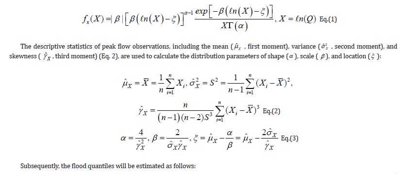
The descriptive statistics of peak flow observations, including the mean
 , first moment), variance
 , second moment), and skewness
 , third moment) (Eq. 2), are used to calculate the distribution parameters of shape (α ), scale ( β ), and location (ξ ):

Subsequently, the flood quantiles will be estimated as follows:
Zp corresponds to the pthquantiles of the standard normal distribution, numerically estimated by the following equation:
The goodness of fit is verified using the Blom empirical probability formula [45]:
where i =1 corresponds to the greatest observation ranked and “n” is the total number of peak flow observations. When the plot of 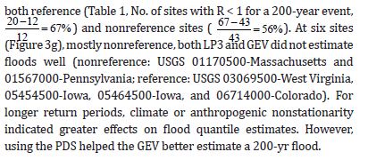 against the anomaly of observations
 falls on the 1:1 line, LP3 reliably estimates flood quantiles [29].
Generalized Extreme Value (GEV)
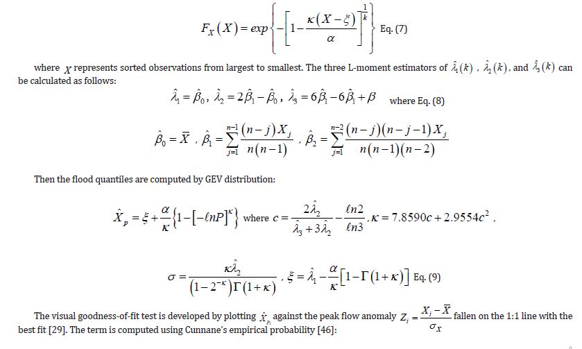
The GEV distribution is represented by the following Cumulative Distribution Functions (CDF):

where X represents sorted observations from largest to smallest. The three L-moment estimators of 

Then the flood quantiles are computed by GEV distribution:

The visual goodness-of-fit test is developed by plotting  against the peak flow anomaly
 allen on the 1:1 line with the
best fit [29]. The term is computed using Cunnane’s empirical probability [46]:

where i =1 for the greatest observation.
Data
Annual maximum flood (AMF)
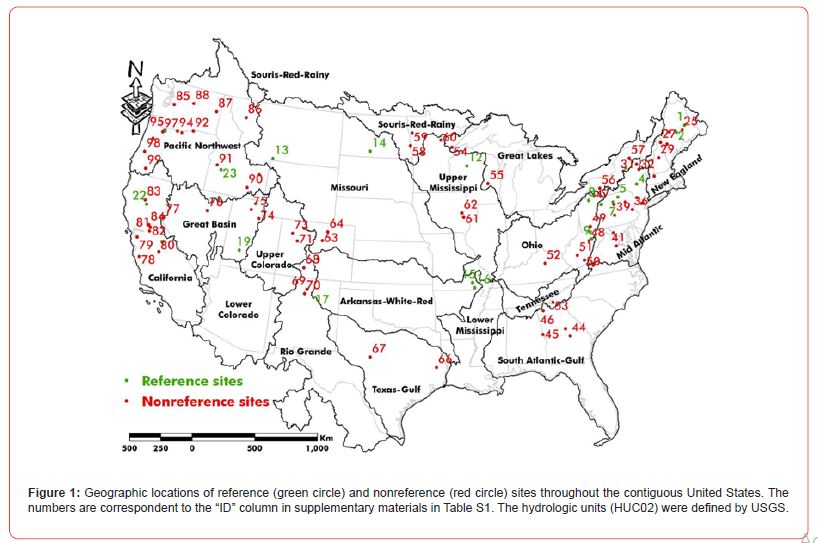
Among 9,067 USGS gauging stations, we selected 99 stations that have more than 100 years of AMF information. Using data from the “Hydro-Climatic Data Network” (HCDN or Gages-II) [47], we classified 24 sites as reference sites situated in undisturbed watersheds, while the remaining 75 were categorized as nonreference sites located in disturbed watersheds. Reference sites experience minimal or no anthropogenic disturbances, whereas nonreference sites exhibit varying levels of land use/cover change, river regulation, and/or reservoir construction [48]. The geographical distribution of stream gauges is illustrated on Figure 1, with additional detailed information about the study sites provided in supplementary materials Table S1. Daily streamflow and peak flow data were obtained from the USGS National Water Information System (NWIS) data repository using the “dataRetrieval” [49] and “dplyr” [50] packages developed in “R.”
Partial duration series (PDS)
The PDS comprises several high flow events rather than just the largest peak flow of each year [16].To ensure compliance with the AMF assumption, it is essential that the selected floods are independent [21]. Developing a PDS from daily mean streamflow data is somewhat subjective. However, as long as the selected peaks represent independent floods and the selection process does not impose too many restrictions [51], can serve as a reliable representation of flood peaks in the region.
In this study, we initially selected flows greater than the minimum peak flow reported in the AMF. Subsequently, we identified the absolute and relative maximums. The final step involved assessing the independence of these maximums. We utilized temporal independence criteria proposed by [26], considering events spaced at least five days apart plus the natural logarithm of drainage area in square miles, as independent flooding events. The length of PDS records for each site is detailed in supplementary materials Table S1. On average, the PDS contained at least five floods in addition to the annual maximum.
Results and discussions
Performance of LP3 and GEV
The performance of a statistical distribution in estimating flood quantiles is assessed through a goodness-of-fit test [29]. When either an LP3 or GEV distribution was fitted to the AMF or PDS, Pearson cross-correlation indicated how accurately the distribution estimated floods with different recurrence intervals. Figure 2 depicts two flood frequency models and the goodness-offit plots for the Connecticut River at Montague City, Massachusetts (USGS 01170500). While both LP3 (Figure 2a) and GEV (Figure 2b) exhibited reliable performance, as evidenced by high correlation coefficients, both distributions missed a few low-frequency floods. This occurred because the goodness of fit primarily evaluated the relative performance of the LP3 or GEV, assigning less weight to the upper and lower tails of the distributions [52]. Therefore, the goodness-of-fit test was supplemented by the ratio (R) of observed to estimated floods to provide a more comprehensive evaluation of the performance of statistical distributions.
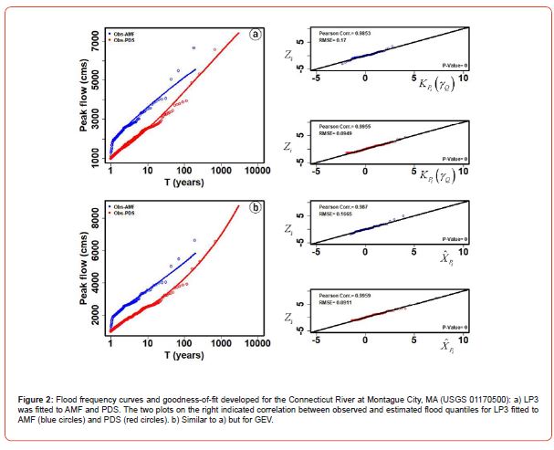
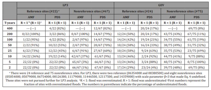
When the ratio fell below one, the distribution performed reliably, indicating that the estimated floods exceeded the corresponding observations. Conversely, a ratio greater than one indicated underestimated flood quantiles, suggesting poor performance of the distribution. We compared the performance of LP3 and GEV with both AMF and PDS at reference and nonreference sites for floods with return periods ranging from two to 400 years. However, in case where either LP3 or GEV performed well with both AMF and PDS, preference should be given to AMF data over PDS, as the development process of a PDS series was subjective.
Two-year flood
LP3 performed well in estimating a two-year flood event with both AMF and PDS information (Figure 3a and Table 1). For regional flood analysis in the Northeast and Pacific Northwest, considering the increase in high-frequency flooding prompted by sea-level rise [53, 54], using GEV with PDS provided better quantile estimates than AMF. However, for the Upper Colorado and northeast of the Great Basin, LP3 outperformed GEV (Figure 3a). Since LP3 demonstrated similar performance with both AMF and PDS, AMF usage was preferred (Table 1). Overall, GEV reliably estimated a two-year flood with PDS information. The distinction between reference and nonreference sites did not affect the performance of LP3, while GEV was sensitive to the conditions of the study sites (Table 1).
Table 1: The ratio (R) of observed peak flows to the corresponding flood quantiles (Obs/Est) estimated by LP3 and GEV distributions for reference and nonreference sites.
Five-year flood
LP3 performed well in estimating a five-year flood with both AMF and PDS (Figure 3b and Table 1). However, the performance of GEV was not spatially consistent. Interestingly, adding more information to a flood series through the use of the PDS alongside AMF did not improve the performance of the GEV and actually worsened it (Table 1). At equal numbers of sites, the GEV with AMF could or could not estimate floods well. Given the uncertainty surrounding the use of GEV for a five-year flood estimation, it appeared that LP3, either with AMF or PDS (with a preference for AMF), was a better choice regardless of site being reference or nonreference (Table 1).
Ten-year flood
For 10-year flooding events, the use of the PDS improved
the LP3 flood quantile estimates compared to the AMF for both
reference and nonreference sites (Table 1, No. of sites with R < 1
for 10-year event,  and nonreference
 sites. Similarly to a five-year flood, the performance of GEV worsened
when using the PDS instead of the AMF (Table 1). The LP3
distribution with PDS data should be utilized for both reference
and nonreference sites, while the use of GEV distribution should
be avoided. At three sites (nonreference: USGS 03284000-Kentucky
and 09239500-Colorado; reference: USGS 04254500-New York),
neither LP3 nor GEV performed well, even with the use of the PDS
instead of the AMF (Figure 3c). Other distributions besides LP3 and
GEV may improve flood estimations for these sites.
Twenty-five-year flood
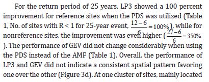
For the return period of 25 years, LP3 showed a 100 percent
improvement for reference sites when the PDS was utilized (Table
1, No. of sites with R < 1 for 25-year event,

 while for
nonreference sites, the improvement was even higher
 ). The performance of GEV did not change considerably when using
the PDS instead of the AMF (Table 1). Overall, the performance of
LP3 and GEV did not indicate a consistent spatial pattern favoring
one over the other (Figure 3d). At one cluster of sites, mainly located in the mid-Atlantic, neither LP3 nor GEV distributions performed
well (Figure 3d). Since in that cluster, the number of reference sites
was greater than nonreference sites, it might imply an increase in
climate nonstationarity for higher flood quantiles in the Northeast
[55], where LP3 and GEV failed to capture the peak flows. A smaller
number of nonreference sites compared to reference sites, where
neither LP3 nor GEV were fitted to peak flow observations, indicated
how climate nonstationarity could be masked by anthropogenic
disturbances in the northeastern U.S. [56].
Fifty-year flood
For 50-year floods, LP3 did not perform well with the AMF
regardless of site conditions (Table 1). Although using the PDS
improved the performance of LP3, the number of sites with R <1
and R > 1 did not indicate significant differences. LP3 might not
be a suitable choice for 50-year flood estimations across the U.S.
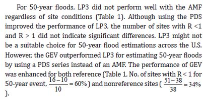
However, the GEV outperformed LP3 for estimating 50-year floods
by using a PDS series instead of an AMF. The performance of GEV
was enhanced for both reference (Table 1, No. of sites with R < 1 for
50-year event,  and nonreference sites
 ).
).
It appeared that GEV could perform well for flood estimations in the Northeast (Figure 3e). Since neither LP3 nor GEV performed well at the following nonreference sites (USGS01076500-New Hampshire, 01434000-New York, 03082500-Pennsylvania, and 08313000-New Mexico), utilizing other distributions besides LP3 and GEV is suggested (Figure 3e). With all those sites being nonreference, it might indicate that, depending on the region of interest, anthropogenic nonstationarity might echo climate nonstationarity [56].
One-hundred-year flood
For a 100-year flood, the PDS did not improve the performance
of LP3 compared to AMF (Table 1). However, using the PDS
instead of the AMF significantly enhanced the performance of
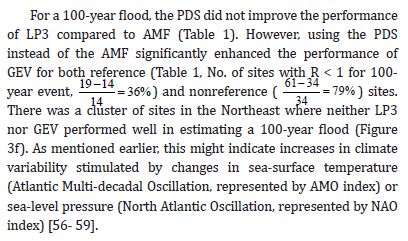
GEV for both reference (Table 1, No. of sites with R < 1 for 100-
year event,  and nonreference
  sites.
There was a cluster of sites in the Northeast where neither LP3
nor GEV performed well in estimating a 100-year flood (Figure
3f). As mentioned earlier, this might indicate increases in climate
variability stimulated by changes in sea-surface temperature
(Atlantic Multi-decadal Oscillation, represented by AMO index) or
sea-level pressure (North Atlantic Oscillation, represented by NAO
index) [56- 59].
Two-hundred-year flood
The 200-year floods showed similar patterns to 100-year
floods (Figure 3g and Table 1). The performance of LP3 was not
significantly improved, even when using the PDS instead of the
AMF. However, the PDS enhanced the performance of the GEV for
both reference (Table 1, No. of sites with R < 1 for a 200-year event,  and nonreference sites
  At six sites
(Figure 3g), mostly nonreference, both LP3 and GEV did not estimate
floods well (nonreference: USGS 01170500-Massachusetts and
01567000-Pennsylvania; reference: USGS 03069500-West Virginia,
05454500-Iowa, 05464500-Iowa, and 06714000-Colorado). For
longer return periods, climate or anthropogenic nonstationarity
indicated greater effects on flood quantile estimates. However,
using the PDS helped the GEV better estimate a 200-yr flood.
Four-hundred-year flood
Flood frequency analysis for a return period of 400 years was only feasible for the PDS since it comprised of at least 350 peak flow observations on average (Table S1). Regardless of whether the sites were reference or nonreference, the GEV considerably better estimated a 400-year flood than the LP3 (Figure 3h and Table 1). At a cluster of sites in the mid-Atlantic, neither GEV nor LP3 accurately estimate a 400-year flood, even when using the PDS instead of the AMF. Similar to a 200-year flood, the confounding effects of changing climate and anthropogenic disturbances were evident in the Northeast, suggesting greater uncertainties in high flood quantile forecasting.
Summary and conclusions
We constructed a PDS from daily streamflow data gathered from 24 reference and 75 nonreference sites across the U.S., each site having more than 100 years of AMF records. Since the PDS provided multiple flooding events per year instead of just the maximum observed peak flow as indicated by the AMF, its inclusion in flood frequency analysis suggested potential improvement in flood quantile estimates. We applied LP3 (product moment) and GEV (L-moment) distributions to both the AMF and PDS. By comparing results between reference and nonreference sites, we aimed to differentiate between climate variations with anthropogenic nonstationarity.
We have summarized the results for distributions suitable for estimating two- to 400-year flooding events in Table 2. We observed that for high-frequency floods with recurrence intervals of two to 10 years, LP3 fitting to the AMF data performed well. However, for longer return periods, the PDS aided in improving the performance of LP3. There was no clear recommendation for an appropriate distribution for a 25-year flood. It appears this return period acted as a transition, replacing the LP3, which reliably estimated shorter period floods of two to 10 years, with the GEV for estimating longer period flooding events. For high flood quantiles of 50-400 years, the performance of GEV was significantly enhanced using the PDS.
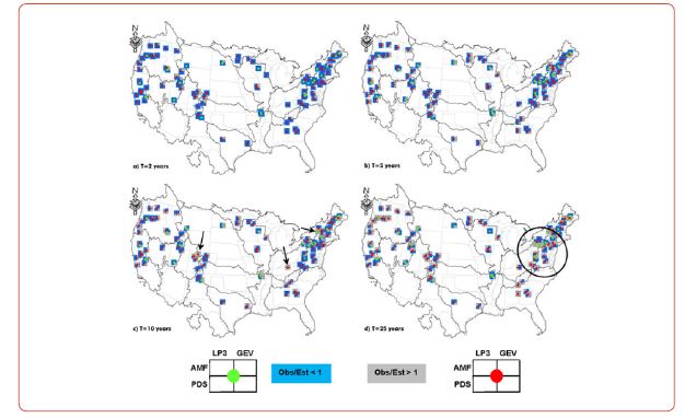
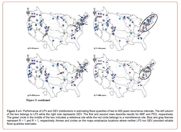
Table 2: Suggested statistical distribution along with appropriate peak flow information for improving flood quantiles estimates across the U.S.

Sites where neither LP3 nor GEV reliably estimated flood quantiles require special attention. This could be indicative of increases in either climate or anthropogenic nonstationarity in the region. One potential solution would be to examine the performance of other distributions introduced for addressing nonstationarity [57]. Poor performance of LP3 or GEV was mainly observed in the Northeast, where climate nonstationarity has affected high flood quantiles in the region [54]. Increases in climate variability could be stimulated by Atlantic circulation patterns [58-61]. Future study should focus on understanding how variations in flood generating mechanisms can affect high and low flood quantile estimates. Reliable flood quantile estimates, considering nonstationarity, help improve flood forecasting, and reduce property damage and loss of life through enhanced infrastructure design, reservoir management, and floodplain determination.
Acknowledgments
Authors would like to acknowledge and extent their gratitude for the support provided by Kansas State University for the current research. The work was conducted from 2018 to 2019, during Dr. Berton’s tenure as a postdoctoral fellow and Dr. Rahmani’s tenure as an assistant professor in the Department of Biological and Agricultural Engineering at Kansas State University.
Conflict of Interest
No Conflict of Interest
Disclaimers
The views expressed in this publication are solely those of the authors and do not necessarily reflect the views of their either formers or current affiliations.
References
- Basso S, Schirmer M, Botter G (2016) A physically based analytical model of flood frequency curves. Geophysical Research Letters 43: 9070-9076.
- Jakob D (2013) Nonstationarity in Extremes and Engineering Design, in: AghaKouchak A, Easterling D, Hsu K, Schubert S, Sorooshian S (Eds.), Extremes in a Changing Climate: Detection, Analysis and Uncertainty, Water Science and Technology Library. Springer, Dordrecht, pp. 363-417.
- Keller L, Rössler O, Martius O, Weingartner R (2018) Delineation of flood generating processes and their hydrological response. Hydrological Processes 32: 228-240.
- Read LK, Vogel RM (2015) Reliability, return periods, and risk under nonstationarity. Water Resources Research 51: 6381-6398.
- Rosner A, Vogel RM, Kirshen PH (2014) A risk-based approach to flood management decisions in a nonstationary world. Water Resources Research 50: 1928-1942.
- Yan L, Xiong L, Guo S, Xu CY, Xia J, et al. (2017a) Comparison of four nonstationary hydrologic design methods for changing environment. Journal of Hydrology 551: 132-150.
- England Jr JF, Cohn TA, Faber BA, Stedinger JR, Thomas Jr WO, et al. (2018) Guidelines for determining flood flow frequency—Bulletin 17C (Report No. 4-B5). Techniques and Methods Reston, VA.
- Shaw SB, Walter MT (2011) Using comparative analysis to teach about the nature of nonstationarity in future flood predictions. Hydrol. Earth Syst. Sci. Discuss 8: 11387-11411.
- Yan L, Xiong L, Liu D, Hu T, Xu CY (2017b) Frequency analysis of nonstationary annual maximum flood series using the time-varying two-component mixture distributions: Time-varying Two-component Mixture Distributions. Hydrological Processes 31: 69-89.
- Luke A, Vrugt JA, AghaKouchak A, Matthew R, Sanders BF (2017) Predicting nonstationary flood frequencies: Evidence supports an updated stationarity thesis in the United States. Water Resources Research 53: 5469-5494.
- Milly PCD, Betancourt J, Falkenmark M, Hirsch RM, Kundzewicz ZW, et al. (2008) Stationarity is dead: Whither water management? Science 319: 573-574.
- Slater LJ, Singer MB, Kirchner JW (2015) Hydrologic versus geomorphic drivers of trends in flood hazard. Geophysical Research Letters 42: 370-376.
- Stephens E, Day JJ, Pappenberger F, Cloke H (2015) Precipitation and floodiness. Geophysical Research Letters 42: 10316-10323.
- Vasiliades L, Galiatsatou P, Loukas A (2015) Nonstationary Frequency Analysis of Annual Maximum Rainfall Using Climate Covariates. Water Resources Management 29: 339-358.
- Yan M, Liu J, Wang, Z (2017) Global Climate Responses to Land Use and Land Cover Changes Over the Past Two Millennia. Atmosphere 8: 64.
- Lang M, Ouarda TBMJ, Bobée B (1999) Towards operational guidelines for over-threshold modeling. Journal of Hydrology 225: 103-117.
- Roth M, Buishand TA, Jongbloed G, Klein Tank AMG, van Zanten JH (2012). A regional peaks-over-threshold model in a nonstationary climate. Water Resources Research 48.
- Adamowski K, Liang GC, Patry GG (1998) Annual maxima and partial duration flood series analysis by parametric and non-parametric methods. Hydrological Processes 12: n1685-1699.
- Archfield SA, Hirsch RM, Viglione A, Blöschl G (2016) Fragmented patterns of flood change across the United States. Geophysical Research Letters 43: 10232-10239.
- Armstrong WH, Collins MJ, Snyder NP (2012) Increased frequency of low-magnitude floods in New England. Journal of the American Water Resources Association 48: 306-320.
- Bezak N, Brilly M, Šraj M (2014) Comparison between the peaks-over-threshold method and the annual maximum method for flood frequency analysis. Hydrological Sciences Journal 59: 959-977.
- Burn DH, Whitfield PH (2017) Changes in cold region flood regimes inferred from long-record reference gauging stations. Water Resources Research 53: 2643-2658.
- Keast D, Ellison J (2013) Magnitude Frequency Analysis of Small Floods Using the Annual and Partial Series. Water 5: 1816-1829.
- Chou C, Chiang JCH, Lan CW, Chung CH, Liao YC, et al. (2013) Increase in the range between wet and dry season precipitation. Nature Geoscience 6: 263-267.
- Seager R, Naik N, Vogel L (2011) Does Global Warming Cause Intensified Interannual Hydroclimate Variability? J. Climate 25: 3355-3372.
- Flynn KM (1982) Guidelines for determining flood flow frequency—Bulletin 17B. U.S. Geological Survey, Office of Water Data Coordination, Reston, Virginia.
- Langbein WB (1949) Annual floods and the partial-duration flood series. Eos, Transactions American Geophysical Union 30: 879-881.
- Nied M, Pardowitz T, Nissen K, Ulbrich U, Hundecha Y, et al. (2014). On the relationship between hydro-meteorological patterns and flood types. Journal of Hydrology 519: 3249-3262.
- Serago JM, Vogel RM (2018) Parsimonious nonstationary flood frequency analysis. Advances in Water Resources 112: 1-16.
- Villarini G, Smith JA, Baeck ML, Krajewski WF (2011) Examining Flood Frequency Distributions in the Midwest U.S. JAWRA Journal of the American Water Resources Association 47: 447-463.
- Berghuijs WR, Woods RA, Hutton CJ, Sivapalan M (2016) Dominant flood generating mechanisms across the United States Geophysical Research Letters 43: 4382-4390.
- Maurer EP, Kayser G, Doyle L, Wood AW (2018) Adjusting Flood Peak Frequency Changes to Account for Climate Change Impacts in the Western United States. Journal of Water Resources Planning and Management 144: 1-12.
- Slater LJ, Villarini G (2016) Recent trends in U.S. flood risk. Geophysical Research Letters 43: 12428-12436.
- Vogel RM, Wilson I (1996) Probability distribution of annual maximum, mean, and minimum stream flows in the united states. Journal of Hydrologic Engineering 1: 69-76.
- Slater LJ, Villarini G (2018) Enhancing the Predictability of Seasonal Streamflow With a Statistical-Dynamical Approach. Geophysical Research Letters 45: 6504-6513.
- Wang W, Lu H, Ruby Leung L, Li HY, Zhao J, et al. (2017) Dam Construction in Lancang-Mekong River Basin Could Mitigate Future Flood Risk From Warming-Induced Intensified Rainfall: Dam Mitigate Flood Risk in Mekong. Geophysical Research Letters 44: 10378-10386.
- Bureau of Reclamation & USACE (2015) Probabilistic Hydrologic Hazard Analysis, in: Best Practices in Dam and Levee Safety Risk Analysis, Training Manual. The Bureau of Reclamation Technical Service Center and the U.S. Army Corps of Engineers Risk Management Center, Denver, Co, p. 20.
- Micevski T, Hackelbusch A, Haddad K, Kuczera G, Rahman A (2015) Regionalisation of the parameters of the log-Pearson 3 distribution: a case study for New South Wales, Australia. Hydrological Processes 29: 250-260.
- Sraj M, Bezak N, Brilly M (2014) Bivariate flood frequency analysis using the copula function: a case study of the Litija station on the Sava River. Hydrological Processes 29: 225-238.
- Bobée B (1975) The Log Pearson type 3 distribution and its application in hydrology. Water Resources Research 11: 681-689.
- Griffis VW, Stedinger JR (2007) Log-Pearson Type 3 Distribution and Its Application in Flood Frequency Analysis. I: Distribution Characteristics. Journal of Hydrologic Engineering 12: 482-491.
- Madsen H, Rasmussen PF, Rosbjerg D (1997) Comparison of annual maximum series and partial duration series methods for modeling extreme hydrologic events: 1. At-site modeling. Water Resources Research 33: 747-757.
- Vogel RM, Fennessey NM (1993) L moment diagrams should replace product moment diagrams. Water Resources Research 29: 1745-1752.
- Stedinger JR, Vogel RM, Foufoula Georgiou E (1993) Frequency analysis of extreme events, in: Maidment, D.R. (Ed.), Handbook of Hydrology. McGraw-Hill, the University of Michigan, p. 1424.
- Blom G (1958) Statistical estimates and transformed beta-variables. John Wiley & Sons, Inc.
- Cunnane C (1978) Unbiased plotting positions — A review. Journal of Hydrology 37: 205-222.
- Falcone J, (2011) GAGES-II: Geospatial attributes of gages for evaluating streamflow (vector digital data). U.S. Geological Survey, Reston, Virginia.
- Lins HF (2012) USGS Hydro-Climatic Data Network 2009 (HCDN–2009) (Fact Sheet). U. S. Geological Survey, Reston, VA.
- Hirsch RM, De Cicco LA (2015) User guide to Exploration and Graphics for RivEr Trends (EGRET) and dataRetrieval: R packages for hydrologic data, Techniques and Methods. U.S. Geological Survey, Reston, VA.
- Wickham H, François R, Henry L, Müller K (2018) dplyr: A Grammar of Data Manipulation, R package version 0.7.6.
- Fahim A, Jean, R (1983) The effect of certain restrictions imposed on the interarrival times of flood events on the Poisson distribution used for modeling flood counts. Water Resources Research 19: 481-485.
- Alila Y, Mtiraoui A (2002) Implications of heterogeneous flood-frequency distributions on traditional stream-discharge prediction techniques. Hydrological Processes 16: 1065-1084.
- Moftakhari HR, AghaKouchak A, Sanders BF, Feldman DL, Sweet W, et al. (2015) Increased nuisance flooding along the coasts of the United States due to sea level rise: Past and future. Geophysical Research Letters 42: 9846-9852.
- Moftakhari HR, AghaKouchak A, Sanders BF, Allaire M, Matthew RA (2018) What Is Nuisance Flooding? Defining and Monitoring an Emerging Challenge. Water Resources Research. 54: 4218-4227.
- Collins MJ (2009) Evidence for changing flood risk in New England since the late 20th century. Journal of the American Water Resources Association 45: 279-290.
- Berton R, Driscoll CT, Chandler DG (2016) Changing climate increases discharge and attenuates its seasonal distribution in the northeastern United States. Journal of Hydrology: Regional Studies 5: 164-178.
- Salas J, Obeysekera J (2013) Revisiting the Concepts of Return Period and Risk for Nonstationary Hydrologic Extreme Events. Journal of Hydrologic Engineering 19: 554-568.
- Berton R, Driscoll CT, Adamowski JF (2017) The near-term prediction of drought and flooding conditions in the northeastern United States based on extreme phases of AMO and NAO. Journal of Hydrology 553: 130-141.
- Collins MJ, Kirk JP, Pettit J, DeGaetano AT, McCown ZS, et al. (2014) Annual floods in New England (USA) and Atlantic Canada: synoptic climatology and generating mechanisms. Physical Geography 35: 195-219.
- Hurrell JW, Deser C (2009) North Atlantic climate variability: The role of the North Atlantic Oscillation. Journal of Marine Systems 78: 28-41.
- Tootle GA, Piechota TC, Singh A (2005) Coupled oceanic-atmospheric variability and U.S. streamflow. Water Resources Research 41: W12408.
Table 3: Description of 24 reference and 75 nonreference study sites with more than 100 years of peak flow information across the contiguous United States.

-
Rouzbeh Berton* and Vahid Rahmani. Improving Low-Frequency Flood Estimation Using the Partial Duration Series Instead of the Annual Maximum Across the United States. Adv in Hydro & Meteorol. 1(5): 2024. AHM.MS.ID.000523.
-
Flood; Climate change; Partial duration series; Annual maximum flood; Log pearson type III; Generalized extreme value; Anthropogenic; Land; Water; Damming
-

This work is licensed under a Creative Commons Attribution-NonCommercial 4.0 International License.


