


 Research Article
Weighted Statistics for Testing Multiple Endpoints in Clinical Trials
Received Date: April 05, 2019; Published Date: May 02, 2019
Abstract
Bonferroni, Holm, and Holm-type stepwise approaches have been well developed for the simultaneous testing of multiple hypotheses in medical experiments. Methods exist for controlling familywise error rates at their preset levels. This article shows how performance of these tests can often be substantially improved by accounting for the relative difficulty of tests. Introducing suitably chosen weights optimizes the error spending between the multiple endpoints. Such an extension of classical testing schemes generally results in a smaller required sample size without sacrificing the familywise error rate and power.
Keywords: Error spending; Familywise error rate; Likelihood ratio test; Minimax; Stepwise testing
Introduction
Many clinical trials and other statistical experiments are conducted to test not one but many hypotheses. Often a decision has to be made on each individual null hypothesis instead of combining them into one composite statement. Most of the clinical trials of new medical treatments have to establish both their safety and efficacy, often involving multiple endpoints or multiple competing treatments [1-4]. For example, recent clinical trials of Prometa, a drug addiction treatment, included testing for multiple side effects as well as multiple criteria of effectiveness such as reduction of craving, improvement of cognitive functions, and frequency of drug abuse [5,6]. Studies of genetic association explore multiple genes and multiple single nucleotide polymorphisms, or SNPs [7-9].
It is still common in applied research to conduct multiple tests, each at a nominal 5% level of significance, and report only those results where significant effects were observed. Anderson [10] estimates that 84% of randomized evaluation articles in diverse fields test five or more outcomes, and 61% test ten or more, but they fail to adjust for multiple comparisons. Clearly, when each hypothesis is tested at a given level α , the probability of committing a Type I error and reporting at least one significant effect is much higher than α even when no effects exist in the population and all the null hypotheses are true.
For this reason, a number of methods for multiple comparisons
have been developed to control a familywise error rate (FWER)
which is the probability of rejecting at least one true null
hypothesis, see [11-14] for the overview. The Bonferroni approach,
due to its simplicity, arguably remains the most commonly used
method of multiple testing. Each individual hypothesis is tested at
a significance level αj, guaranteeing that FWER ≤α as long as
Σαj≤α . However, the underlying Bonferroni (Boole) inequality
 is not sharp, leaving room for improvement
Enhancing the Bonferroni method, Holm [15] proposed a scheme based on the ordered p-values. Developing upon Holm’s idea, step-up and step-down methods for multiple testing have been developed for non-sequential [11,16-19] and most recently, sequential experiments [20-23]. These Holm-type methods (also called stepwise for testing marginal hypotheses in the order of their significance) allow to use higher levels of αj leading to increased power, while still controlling FWER.
These stepwise methods and most of the other approaches to multiple tests do not account for different levels of difficulty of the participating tests, or proximity between null hypotheses and their corresponding alternative hypotheses. Why should we take this into account when designing statistical experiments?
Example. As a simple example, consider simultaneous testing of three endpoints in a clinical trial, where the null parameter differs from the alternative parameter by 0.35 standard deviations in the first test, by 0.30 standard deviations in the second test, and by 0.25 standard deviations in the third test. What sample size suffices for controlling FWERs at α = 0.05and β = 0.10 , assuming normal measurements with known standard deviations?
Following the standard Bonferroni approach, we conduct each
test atαj= α/ 3 j and βj= β / 3 , and this requires 129 observations
to conduct the first test, 175 for the second test, and 252 for the
third test, computed by the formula  , where
δjis the distance between the null and alternative parameters
measured in respective standard deviations. It is not surprising
that the easiest test #1 (because it is easier to detect a larger
difference between the null and the alternative hypotheses)
requires the smallest sample size. Imagine, however, that all three
data sequences are obtained from the same sampling units such
as patients each answering three questions in their questionnaire
or measuring concentrations of three substances in their blood
samples. Then we still need to sample all 252 patients to guarantee
the FWER control!
, where
δjis the distance between the null and alternative parameters
measured in respective standard deviations. It is not surprising
that the easiest test #1 (because it is easier to detect a larger
difference between the null and the alternative hypotheses)
requires the smallest sample size. Imagine, however, that all three
data sequences are obtained from the same sampling units such
as patients each answering three questions in their questionnaire
or measuring concentrations of three substances in their blood
samples. Then we still need to sample all 252 patients to guarantee
the FWER control!
Since three tests had differing levels of difficulty, the uniform error spending (α / 3,α / 3,α / 3) and (β / 3,β / 3,β / 3) was not optimal. As it is shown in Theorem 3.1 of De and Baron [24], the asymptotically most difficult test should optimally receive almost the entire allowed error probability, in the extreme case under the Pitman alternative. We do not have a limiting case here, but there is ample room for improvement. A better error spending is (α1 = 0.006,α2 = 0.014,α3 = 0.030) and (β1 = 0.011,β1 = 0.028,β1 = 0.0610) . In this case, a sample of 189 patients instead of 252 is sufficient, for a pure 25% saving, using the (generalized) Bonferroni procedure.
Stepwise procedures have a potential to increase this saving even further. However, the Holm method does not distinguish between “easy” and “difficult” tests. The Holm-adjusted levels of significance areα / d,α / (d −1),....,α , regardless of the tested null and alternative parameter values and their proximity. In this paper, we generalize the Holm method to allow higher than Bonferroni significance levels and, at the same time, to account for the difficulty levels, which results in reduced required sample sizes.
The key in this optimization is minimaxity of the optimal error spending. Indeed, the sample size is determined by the test that requires the largest number of patients, because we need enough data to reach decision for each individual hypothesis. Minimizing the overall sample size implies minimizing the largest sample size among individual tests, and thus, the solution of this problem is minimax. The form of this solution is an equalizer rule [25], defined in this case as such error spending that equalizes the required sample sizes.
The key in this optimization is minimaxity of the optimal error spending. Indeed, the sample size is determined by the test that requires the largest number of patients, because we need enough data to reach decision for each individual hypothesis. Minimizing the overall sample size implies minimizing the largest sample size among individual tests, and thus, the solution of this problem is minimax. The form of this solution is an equalizer rule [25], defined in this case as such error spending that equalizes the required sample sizes.
We show in this article how the optimal solution can be calculated and derive Bonferroni and Holm-type procedures that follow this minimax rule. Even for the tests where the levels of difficulty are close (but not equal), these new methods may result in substantial cost saving.
Problem Formulation
Consider a sample of multidimensional measurements
( X1,,, Xn) , where each d
i  its j-th component X ij the j-th
endpoint for the i-th patient, has a marginal distribution with
density
its j-th component X ij the j-th
endpoint for the i-th patient, has a marginal distribution with
density  with respect to some probability measure μ j andθ(1) ,....θ (d ) are parameters of interest. Components of the same
observed vector may be correlated; however, we do not assume
any knowledge of their joint distribution and use only the marginal
distributions for our statistical inference. For example, Xi may be
vital signs measured on the i-th patient or responses of the i-th
survey participant.
with respect to some probability measure μ j andθ(1) ,....θ (d ) are parameters of interest. Components of the same
observed vector may be correlated; however, we do not assume
any knowledge of their joint distribution and use only the marginal
distributions for our statistical inference. For example, Xi may be
vital signs measured on the i-th patient or responses of the i-th
survey participant.
The goal is to conduct d tests of

controlling Type I and Type II familywise error rates

where Τ ⊂{1,...., d}is the index set of true null hypotheses, and F=T is its complement, the index set of false nulls.
In this article, we seek efficient non-sequential multiple testing procedures for (2.1). Under conditions
FWERI ≤α and FWERII ≤ β (2.3)
we aim at minimizing the required sample size n (and therefore, the overall cost of the experiment) by using efficient test statistics and optimal error spending.
A Clinical Trial of Flector
To see the size of potential saving, let us consider a simple case of testing means of two normal distributions

based on a sample of bivariate normal random vectors X1,..., Xn with mean (θ(1) ,θ(2)) known standard deviations σ(1) ,σ (2) , and unknown correlation ρ .
Such a situation appeared, for example, in the design of a recent clinical trial of Flector, a patch containing a topical treatment of ankle sprains. Patients were randomized to three groups - a brand name Flector patch, its generic version, and placebo. The trial was designed to support two statements - (1) that the generic patch is as effective as the brand name, and (2) that both of them are better than placebo. Thus, test 1 establishes bioequivalence of two treatments and test 2 establishes efficacy, where the two active treatment arms are merged and compared against the placebo arm. By the standard protocol, bioequivalence is established if r, the ratio of three-day mean pain reduction levels between generic and brandname patients, has a 90% confidence interval entirely within the interval [0.8, 1.25]. Since we are actually interested in confirming that the generic patch is at least as efficient as the Flector patch, both tests can be reduced to the form (3.1), whereθ(1) = r (testing r = 0.8 vs r = 1.0) and θ(2) = Δ = μT −μP is the difference in the mean pain reduction levels between the merged active treatment group and the placebo group (testing Δ = 0 vs Δ = 4 ) Standard deviations σ (1) = 0.373 and σ(2) =19.01estimated from the previous studies of similar products such as Lionberger et al. (2011), imply the standardized distances

and thus, the test of efficacy appears more difficult than the test of bioequivalence. As conducted at the actual marginal levels of α1 = 0.05,β1 = 0.01,α2 = 0.05,β2 = 0.14 these tests required n = 169 patients in each treatment arm (the actual trial included 170 patients in each arm), and with this sample size, both test statistics appeared approximately normal.
Chosen to control individual error probabilities, this sample size actually suffices to keep the Type I familywise error rate at the same level 1 α = 0.05. The optimal error spending in this case is
0.05 = 0.00002+ 0.04998. (3.2)
That is, it is most efficient to split α1 = 0.05very unevenly into α1 = 0.00002and α2 = 0.04998 , due to different levels of difficulty. In other words, with one test being so much “easier” than the other, the whole trial can be planned to test the most difficult hypothesis, whereas the “easier” test can then be conducted practically at no additional expense, matching the result in Theorem 3.1 of De and Baron [24].
Such an unequal error spending is explained in Figure 1. We see that almost all the error is spent on the more difficult test if δ1 /δ2 ∉ (0.5, 2.0) i.e., one test is at least twice as difficult as the other (Figure 1).

A simple computation shows that uniform α -spending for testing (3.1) with the listed β1,2 and FWERI of α = 0.05 requires a sample of size n = 210 in each treatment arm whereas n = 169 suffices with error spending (3.2), using the Bonferroni method
Table 1 shows the optimal error spending of α1 = 0.05 and β1 = 0.10 for the case of d = 2 tests, with different levels of difficulty δ1,2 . Naturally, the optimal split of δ and β becomes more uneven when δ2 differs substantially from δ1 . For testing θ = 0.25 against θ = 0.3 , the more difficult test already receives more than twothirds of the allowed error probability. When δ2 /δ1 > 2 the required sample size N = 138 is the same as one needs to conduct just a single test of H(1)0. Thus, optimal error spending allows to add substantially easier tests at practically no extra cost, while controlling the familywise error rates. For the comparison, the uniform error spending and the standard Bonferroni adjustment for multiple comparisons requires N = 201 for each of these tests.
The Holm-type stepwise approach provides further saving (Table 1).
Table 1: Optimal error spending of α1 = 0.05and β1 = 0.10 for two tests and the required sample size N.

Minimax Error Spending
Minimax problem and equalizer solution
The optimal error spending in Section 3 is calculated by attaining the same sample size that is required to conduct each test in (3.1).
Indeed, as we know (for example, from [26], ch. 4), the minimum sample size needed to test the j-th normal mean at levels αj and β jis

where  andΦ(⋅) is a standard normal cdf.
A conclusive decision on each of d tests requires a sample size
n=max (nj). Thus, minimization of the required sample size,
minmax (nj) is a minimax problem, and its solution is an equalizer
rule (Berger, 1985, ch. 5), which is such error spending { αsub>j, βsub>j}
that yields
andΦ(⋅) is a standard normal cdf.
A conclusive decision on each of d tests requires a sample size
n=max (nj). Thus, minimization of the required sample size,
minmax (nj) is a minimax problem, and its solution is an equalizer
rule (Berger, 1985, ch. 5), which is such error spending { αsub>j, βsub>j}
that yields
n1 = n2 = nd (4.2)
intuitively, optimality of the equalizer testing scheme is natural. Consider error probabilities αj, β j that correspond to unequal sample sizes nj given by (4.1). Then, slowly incrementing error probabilities αj and βj that correspond to the largest sample size nj at the expense of smaller sample sizes, we reduce the overall sample siz n = max (nj). The only situation when such reduction is no longer possible is when all nj are equal, following the (generalized) Bonferroni approach, this minimax problem reduces to solving (4.2) in terms of {αj, β j } and minimizing the common nj among all the existing solutions, subject to Σαj =α and Σβj = β For the tests of normal means, a convenient solution, close to being minimax, is

where cα is the solution of equation  and cβ solves
  . These equations have unique solutions
because the function
. These equations have unique solutions
because the function  is continuous and
monotonically decreasing from d/2 ≥ 1 at t = 0 to 0 at t = +∞
. It follows from (4.1) that error spending (4.3) is an equalizer,
although it is the optimal equalizer only when α = β . Why is there
more than one equalizer solution? We are choosing (2d) marginal
significance levels {αj, β j} for j =1,.....,d under two constraints
on Σαj and Σβj
Additional (d − 1) constraints appear in (4.2).
Therefore, we have (d+1) equations and (2d) variables to choose,
giving us at least one degree of freedom for all d ≥ 2 and a room to
minimize the common sample size nj .
is continuous and
monotonically decreasing from d/2 ≥ 1 at t = 0 to 0 at t = +∞
. It follows from (4.1) that error spending (4.3) is an equalizer,
although it is the optimal equalizer only when α = β . Why is there
more than one equalizer solution? We are choosing (2d) marginal
significance levels {αj, β j} for j =1,.....,d under two constraints
on Σαj and Σβj
Additional (d − 1) constraints appear in (4.2).
Therefore, we have (d+1) equations and (2d) variables to choose,
giving us at least one degree of freedom for all d ≥ 2 and a room to
minimize the common sample size nj .
General distribution and Bahadur efficiency
For non-normal distributions, computation of the exact sample size necessary to attain a given significance level and power is “extremely difficult or simply impossible”, hence, a symptotics are being used (Nikitin, 1995, sec. 1.1) [27]. For distributions that are approximately normal, this approximation yields a rather accurate estimation of the necessary sample size [28] (Dzhungurova and Volodin, 2007). Then, error spending (4.3) is nearly optimal, and sample size (4.1) is nearly sufficient for the control of FWERI and FWERII at levels α and β . For the general case, the asymptotic result of Bahadur [29] about p-value p(j) of the j-th test states that

where  is the Kullback-Leibler information
number between H(j)Aand H(j)0. Equality in (4.4) is attained by
the likelihood ratio test (LRT) that rejects H(j)0 for large values of
statistic
is the Kullback-Leibler information
number between H(j)Aand H(j)0. Equality in (4.4) is attained by
the likelihood ratio test (LRT) that rejects H(j)0 for large values of
statistic

making this test Bahadur asymptotically optimal (Bahadur, 1967, part II). Since our minimax problem is solved by an equalizer, and since the decision on each test is determined by comparing p-values p(j) with marginal significance levels αj, this suggests to choose the error spending αj with log( αj) proportional to K(j)A In other words, the Bonferroni procedure for multiple testing that is based on log-likelihood ratio statistics (4.5) for each marginal test, with error spending

cα being the unique solution  is
asymptotically optimal in Bahadur sense, and it controls the Type I
familywise error rate at level α [30-35]. Similarly, the Type II error
spending
is
asymptotically optimal in Bahadur sense, and it controls the Type I
familywise error rate at level α [30-35]. Similarly, the Type II error
spending  with cβ solving
  controls FWERII.
If a sample is sufficiently large, the multiple testing
procedurewith the introduced α - and β -spending controls
both familywise error rates simultaneously. To see this, we notice
that in order to control the probability of Type I error, each
marginal LRT rejects the corresponding null hypothesis H(j)0 if
 .
.
By Chebyshev’s inequality,

as n → ∞ for any  hence aj(n ) → −∞ .

henceaj( n) ≤ bj(n) for sufficiently large n, which implies that FWERI ≤α and FWERII ≤ β
Generalized Holm method
Instead of comparing marginal p-values p(j) with αj, Σαj =α Holm [23] (1979) proposed to compare the ordered p-values

against α levels  that are
generally larger, with the sum Σαj >α Choosing larger α -levels
increases the power of tests, or, given the same power, they require
a smaller sample. Then, the null hypotheses H(j)0 corresponding
to the ordered p-values are arranged in the same order, and
that are
generally larger, with the sum Σαj >α Choosing larger α -levels
increases the power of tests, or, given the same power, they require
a smaller sample. Then, the null hypotheses H(j)0 corresponding
to the ordered p-values are arranged in the same order, and  are rejected, where
  . These
rejected hypotheses correspond to m most significant p-values.
. These
rejected hypotheses correspond to m most significant p-values.
This multiple testing procedure controls FWERI ≤α [15] (Holm, 1979).
Holm’s method does not account for different levels of difficulty of tested hypotheses. However, it can be generalized to allow optimal solutions similar to (4.6) in the following way [36-41].
Let us order the Kullback Leibler information numbers
 under the null hypotheses
  under the alternatives H(j)A. Then, let ak be the unique solution of
the equation
under the alternatives H(j)A. Then, let ak be the unique solution of
the equation

Also, consider statistics
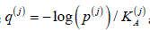 and order them,
q[1] ≥ .... ≥ q[d ] .This order may differ from the ordering of p-values
p[ j] .In the new multiple testing procedure, we compare the ordered
values q[ j] against the corresponding critical values j a . Like Holm’s
method, the null hypotheses
and order them,
q[1] ≥ .... ≥ q[d ] .This order may differ from the ordering of p-values
p[ j] .In the new multiple testing procedure, we compare the ordered
values q[ j] against the corresponding critical values j a . Like Holm’s
method, the null hypotheses  , corresponding to
the ordered q[ j] , are rejected for
, corresponding to
the ordered q[ j] , are rejected for  and all
H(j)0 are accepted (not rejected) if q[j] < aj. for all j. This type of a
multiple testing procedure is step-down because it tests marginal
hypotheses in steps, moving from the most significant q-value to
the least significant one, rejecting null hypotheses one at a time,
and accepting all the remaining hypotheses once any one of them
fails to be rejected.
and all
H(j)0 are accepted (not rejected) if q[j] < aj. for all j. This type of a
multiple testing procedure is step-down because it tests marginal
hypotheses in steps, moving from the most significant q-value to
the least significant one, rejecting null hypotheses one at a time,
and accepting all the remaining hypotheses once any one of them
fails to be rejected.
We show that this multiple testing scheme controls the Type I familywise error rate. First, we notice that the critical values aj are also arranged in a non-decreasing order.
Lemma 1. The critical values k a given as solutions of (4.7) satisfy the inequality, a1 ≥.... ≥ ad.
Proof. If ak > ak−1 for some k = 2, . . . , d, then we arrive at a contradiction,

Theorem 1. The proposed step-down multiple testing procedure with critical values aj given by (4.7) for weighted p-values q[j] controls the Type I familywise error rate, FWERI ≤α
Proof. The proof follows the general idea of Holm [15], adapted
to weighted p-values q[j] and error spending (4.7). Considering the
ordered null hypotheses H(j)0 , let J be the first index of a true null
hypotheses,  . In particular, it implies that the first (J −1) null hypotheses are false. Hence, the number of false hypotheses
F ≥ J −1.
. In particular, it implies that the first (J −1) null hypotheses are false. Hence, the number of false hypotheses
F ≥ J −1.
The next fact to notice is that at least one Type I error occurs
if and only if H(j)0 is rejected. Indeed, acceptance Of
H(j)0 means acceptance of all hypotheses
H(j)0 for j > J, and since all  are false, there will be no
Type I errors in this case. Therefore,


Here, the last inequality in (4.9) follows from Lemma 1; (4.10)
from the definition of q(j) the first inequality in (4.11) from the
inequality  (for example, from (1.2.1) of Nikitin,
1995) [29]; the second inequality of (4.11) from the increasing
order of K[j] ; and the remainder of (4.11) follows from (4.7) with
k = F +1 = d − τ +1.
(for example, from (1.2.1) of Nikitin,
1995) [29]; the second inequality of (4.11) from the increasing
order of K[j] ; and the remainder of (4.11) follows from (4.7) with
k = F +1 = d − τ +1.
Naturally, when all tests have the same difficulty level, in terms
of 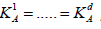 , then equation (4.7) is
solved by 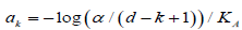 and the generalized
Holm procedure becomes the standard Holm’s as a special case.
and the generalized
Holm procedure becomes the standard Holm’s as a special case.
As another extreme, suppose that one test is much more difficult
than the other tests, namely, 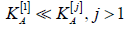 Then equation (4.7)
is approximated by
Then equation (4.7)
is approximated by

from where 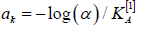
Comparison
An extensive study of different scenarios may be required in order to evaluate the range of saving brought by each multiple testing method – Holm-type stepwise versus Bonferroni, weighted versus unweighted, and sequential versus non-sequential, for various distributions. Here, we just consider an illustrative example.
Consider testing two hypotheses about normal means. Observed
is a sample of random vectors 

Table 2: Required sample size E(T) for sequential multiple testing procedures. The standard Bonferroni and Holm type stepwise tests are compared with their optimized versions designed under minimax error spending.

When the two tests have different levels of difficulty, the optimal error spending brings considerable cost saving, see Table 2. Smaller sample sizes due to the proposed minimax error spending method are seen in columns “Generalized Bonferroni”, compared to the standard Bonferroni method, and “Weighted Stepwise”, compared to the standard stepwise Holm method (Table 2).
The weighting approach brings no saving for the case when
 , when the two tests have the same level of difficulty.
The proposed method is only efficient when tests have different
difficulty levels. Saving due to minimax error spending increases
as the difference between two tests increases. When the test of
, when the two tests have the same level of difficulty.
The proposed method is only efficient when tests have different
difficulty levels. Saving due to minimax error spending increases
as the difference between two tests increases. When the test of
 is five times as difficult as the test of
 the minimax approach requires 443
fewer patients (34% saving) to conduct the Bonferroni procedure,
and 190 fewer patients (18% saving) to conduct stepwise testing.
the minimax approach requires 443
fewer patients (34% saving) to conduct the Bonferroni procedure,
and 190 fewer patients (18% saving) to conduct stepwise testing.
Acknowledgement
Research of both authors at American University was funded by the National Science Foundation.
Conflict of interest
No conflict of interest.
References
- O’Brien PC (1984) Procedures for comparing samples with multiple endpoints. Biometrics 40: 1079-1087.
- Pocock SJ, NL Geller, AA Tsiatis (1987) The analysis of multiple endpoints in clinical trials. Biometrics 43: 487-498.
- Tang DI, NL Geller (1999) Closed testing procedures for group sequential clinical trials with multiple endpoints. Biometrics 55: 1188-1192.
- Wassmer G, W Brannath (2016) Multiple testing in adaptive designs. In Group Sequential and Confirmatory Adaptive Designs in Clinical Trials, Springer, pp. 231-239.
- Urschel HC, LL Hanselka, M Baron (2011) A controlled trial of flumazenil and gabapentin for initial treatment of methylamphetamine dependence. J Psychopharmacology 25(2): 254-262.
- Urschel HC, LL Hanselka, I Gromov, L White, M Baron (2007) Open-label study of a proprietary treatment program targeting type a-aminobutyric acid receptor dysregulation in methamphetamine dependence. Mayo Clinic Proceedings 82(10): 1170-1178.
- Hendricks AE, J Dupuis, MW Logue, RH Myers, KL Lunetta (2014) Correction for multiple testing in a gene region. Eur J Hum Genet 22(3): 414-418.
- Babron MC, A Etcheto, MH Dizier (2015) A new correction for multiple testing in gene–gene interaction studies. Annals of Human Genetics 79(5): 380-384.
- Sul JH, T Raj, S de Jong, PI de Bakker, S Raychaudhuri, et al. (2015) Accurate and fast multiple-testing correction in eQTL studies. The American Journal of Human Genetics 96(6): 857-868.
- Anderson ML (2012) Multiple inference and gender differences in the effects of early intervention: A reevaluation of the Abecedarian, Perry Preschool, and Early Training Projects. Journal of the American Statistical Association.
- Benjamini Y, F Bretz, S Sarkar (2004) Recent Developments in Multiple Comparison Procedures. Beachwood, Ohio: IMS Lecture Notes - Monograph Series.
- Dmitrienko A, AC Tamhane, e Bretz F (2010) Multiple Testing Problems in Pharmaceutical Statistics. Boca Raton, FL: CRC Press, USA.
- Hsu J (1996) Multiple comparisons: theory and methods. CRC Press.
- Bretz F, T Hothorn, P Westfall (2016) Multiple comparisons using R. CRC Press.
- Holm S (1979) A simple sequentially rejective multiple test procedure. Scand J Stat 6(2): 65-70.
- Benjamini Y, Y Hochberg (1995) Controlling the false discovery rate: a practical and powerful approach to multiple testing. J Royal Stat Soc 57(1): 289-300.
- Hochberg Y (1988) A sharper Bonferroni procedure for multiple tests of significance. Biometrika 75(4): 800-802.
- Lehmann EL, JP Romano, JP Shaffer (2012) On optimality of stepdown and step up multiple test procedures. In Selected Works of EL Lehmann, Springer, pp. 693-717.
- Sarkar SK (2002) Some results on false discovery rate in stepwise multiple testing procedures. Ann Stat 30(1): 239-257.
- Bartroff J, TL Lai (2010) Multistage tests of multiple hypotheses. Communications in Statistics - Theory and Methods 39: 1597-1607.
- De S, M Baron (2012b) Step-up and step-down methods for testing multiple hypotheses in sequential experiments. J Statist Plann Inference 142: 2059-2070.
- Bartroff J, J Song (2014) Sequential tests of multiple hypotheses controlling type i and ii familywise error rates. Journal of Statistical Planning and Inference 153: 100-114.
- De S, M Baron (2015) Sequential tests controlling generalized familywise error rates. Statistical Methodology 23: 88-102.
- De S, M Baron (2012a) Sequential Bonferroni methods for multiple hypothesis testing with strong control of familywise error rates I and II. Sequential Analysis 31(2): 238-262.
- Berger JO (1985) Statistical Decision Theory. New York, NY: Springer- Verlag, USA.
- Jennison C, BW Turnbull (2000) Group sequential methods with applications to clinical trials. Boca Raton, FL: Chapman & Hall.
- Nikitin Y (1995) Asymptotic efficiency of nonparametric tests. Cambridge University Press.
- Dzhungurova OA, IN Volodin (2007) The asymptotic of the necessary sample size in testing the hypotheses on the shape parameter of a distribution close to the normal one. Russian Mathematics 51(5): 44-50.
- Bahadur RR (1967) Rates of convergence of estimates and test statistics. The Annals of Mathematical Statistics 38(2): 303-324.
- Baillie DH (1987) Multivariate acceptance sampling - some applications to defence procurement. The Statistician 36(5): 465-478.
- Bartroff J (2014) Multiple hypothesis tests controlling generalized error rates for sequential data. arXiv preprint arXiv:1406.5933.
- Blomquist J (2015) Multiple inference and market integration: An application to swedish fish markets. Journal of Agricultural Economics 66(1): 221-235.
- Borovkov AA, AA Mogulskii (2001) Limit theorems in the boundary hitting problem for a multidimensional random walk. Siberian Mathematical Journal 42(2): 245-270.
- Govindarajulu Z (2004) Sequential Statistics. World Scientific Publishing Co, Singapore.
- Hamilton DC, ML Lesperance (1991) A consulting problem involving bivariate acceptance sampling by variables. Canadian J Stat 19: 109-117.
- Landis WG (2003) Twenty years before and hence; ecological risk assessment at multiple scales with multiple stressors and multiple endpoints.
- Lionberger DR, E Joussellin, A Lanzarotti, J Yanchick, M Magelli (2011) Diclofenac epolamine topical patch relieves pain associated with ankle sprain. J Pain Res 4: 47-53.
- Park J, CH Jun (2015) A new multivariate EWMA control chart via multiple testing. Journal of Process Control 26: 51-55.
- Tartakovsky AG, IV Nikiforov, M Basseville (2014) Sequential Analysis: Hypothesis Testing and Change-Point Detection. Chapman & Hall/CRC.
- Wald A (1947) Sequential Analysis. New York: Wiley, USA.
- Yang Z, X Zhou, P Zhang (2015) Centralization and innovation performance in an emerging economy: testing the moderating effects. Asia Pacific Journal of Management 32(2): 415-442.
-

This work is licensed under a Creative Commons Attribution-NonCommercial 4.0 International License.


