Volatility Forecasting Scalable Oncological Signatures by Temporally Denoising Quadratic Heteroscedasticity in A Platykurtic Student T-Distributed Thick-Tailed Non-Asymptotical Regression Model Output for Optimizing Social Messaging AI-Infused Smartphone Applications for Targeting County-Level Hot Spots of Leukemia Patient Households in Florida

Introduction

According to the Leukemia & Lymphoma Society, an estimated 456,481 people in the United States are living with or in remission from leukemia [1]. Advances in both diagnosis and treatment— such as the use of BCR-ABL tyrosine kinase inhibitors for Chronic Myeloid Leukemia and the identification of disease-associated molecular defects in Acute Myeloid Leukemia—have significantly improved patient outcomes [2,3]. However, many questions about oncological treatment remain unresolved, including models for timing and dosage scheduling, as well as methods for preventing and treating treatment failure. Regression models are widely used in oncology to predict outcomes, assess risk, and understand the relationships between various factors and cancer-related events. Examples of regression-related models published in the literature include those for primary cerebellar lymphoma [4] and testicular cancer [5]. Hematopoiesis [6]. In some cases, regression models have offered insights into the molecular pathogenesis of some cancers [7].

In other literature contributions, regression models have helped medical deciion-making; for example, in identifying which patients are at sufficiently high risk of recurrence to warrant toxic or expensive treatment [8]. Identification of major sociodemographic and landscape topographic determinants can facilitate the design of further trials, aid in inter-trial comparisons, and guide the counseling of individual patients at the county, zip code, and household levels. Unfortunately, the results of different oncological regression models currently employed in the literature may not provide a precise framework for clinicians and other research collaborators to study leukemia genesis and treatment strategies. Although regressively modeling temporal, stratified, capture point sampled estimator determinants can heuristically optimize diagnosis and treatment of oncological processes by interpolating county, zip code stratifiable, capture point signatures. The residual output from these paradigms has not been checked for violations of regression assumptions in time.

Violations of time-sensitive regression assumptions [e.g., non-Gaussian heteroscedastic error variance] occur when the data do not meet the model’s requirements, leading to unreliable results. Key assumptions in predictive, time series, regression-related, oncological capture point modelling include linearity, independence of errors, homoscedasticity (constant variance), and normality of errors. Violations can result in inaccurate coefficient estimation, [e.g., inability to differentiate Chronic Lymphocytic Leukemia (CLL), unreliable hypothesis testing, and poor model predictions [e.g., falsely targeted county zip code, aggregation/non-aggregation (hot/spots/cold spots) of potential CLL)] which can delay treatment, allowing the disease to progress and become more difficult to treat. Furthermore, these regression violations would disallow regressively delineating geographic locations [i.e., geolocations of potential CLL or other oncological patients] when implementing a targeted county-level, prevention social media messaging platform, as the prognostications would be mis-specified [i.e., pseudo-R2 probably estimates of zip code, location regressively forecasted would reveal a falsely targeted georeferenced hot spot].

The accuracy of targeted county and zip code-level prevention social media messaging platform data transfer in AI-ML, mobile, interactive smartphone applications (apps) can vary significantly depending on network conditions, server response times, optimization, and device performance. Currently, selective search engines embedded in mobile devices, such as iOS health apps, merge data based on engineered low-level features and have an order of magnitude of up to 91.3 seconds per information text in a CPU implementation [9]. Faster Regional Convolutional Neural Network [R-CNN] enables end-to-end detector training on shared convolutional features and shows compelling accuracy and speed using Gaussian non-heteroscedastic, non-multicollinear, regressed time series, county, zip code stratified, non-zero autocorrelated, georeferenced estimator determinants [10]. Real-time R-CNN integration works almost instantly, in contrast to typical batch processing, which collects and processes data in predetermined chunks. This implies that intelligent, real-time retrieved smartphone health data can be gathered, retrieved, shared, and preserved in milliseconds, enabling the prompt diagnosis and rehabilitation of oncological processes.

Currently, mobile oncological-related health apps can only employ fixed regression non-time series forecast models for various applications due to the non-availability of real-time oncological-associated regressable data. This can lead to misspecifications in time. For example, non-inclusion of real-time vital regressed data in oncological sampled stratified time series, dependent estimator determinants [e.g., sociodemographic and land use land cover [LULC] capture point signatures, etc.] can cause falsely targeted georeferenced hot and cold spots of potential leukemia patient households. Introduced a Region Proposal Network (RPN) that shares full-image real-time convolutional features within an infused, intelligent, AI-ML detection network in an interactive, continuously self-learning smartphone, mobile app for prediction cost-free region proposals [e.g., signature interpolated regression maps for intervention protocols]. The interactive app may be usable for implementing social messaging for oncological patients at the county, zip code level, using Gaussian time series regression models.

A method is presented to rectify an empirical georeferenced, interpolated, time series, regressed dataset of multicollinear, non-Gaussian, heteroscedastic, zero, autocorrelated county, zip code level, sampled, oncological-related, stratified estimator determinants within a Markovian semiparametric, eigen-Bayesian non-frequentist framework. We intended to heuristically optimize temporal signature capture point interpolation of sampled, georeferenced, regressed, county-level, zip code, stratifiable oncological- related, LULC, and sociodemographic signatures so that they would be capable of handling everything a penalized generalized linear model [GLM] can handle [e.g., estimator determinant, variance error-free Gaussian, non-multicollinear distributional flexibility and credibility]. We assumed a subset of signatured, capture point, georeferenceable, non-erroneous, non-zero autocorrelated, temporal model regression functionalities could be incorporated into a semi-parametric, eigen-Bayesian, prognosticative, non-frequentist Markovian, model framework disturbance-free [i.e., “non-heteroscedastically”].

If an empirical sampled, georeferenced, oncological-related regressed dataset of empirical sampled, signature, estimator determinants can be treated for violations of regression assumptions in time, the forecasts may be employed to heuristically optimize targeting oncological-related, social media messaging prevention and treatment protocols, which may be parsimoniously infusible into a real-time, mobile, AI-ML infused iOS app dashboard. This may allow robustifying capture point forecast mapping and prioritizing potential leukemia patients at the household, county, and zip code levels. The benefits of homoscedastic, non-asymptotical, time series, non-zero autocorrelatable, Gaussian, non-multicollinear, oncological-related, regressively forecasted data capture points in terms of their accuracy and intuitiveness should include optimal predictive power for precision forecast mapping. This would also include implementing a Statewide social media leukemia prevention messaging platform.

Presented two space-time model specifications, one based upon the generalized linear mixed model (GLMM), and the other upon semi-parameterized, Moran, eigenvector, eigen-Bayesian, non-frequentist, Markovian, eigen-spatialized filters for testing non-asymptoticalness, latent homoscedasticity, Gaussian, zero, autocorrelation, and residual non-multicollinearity in an empirical stratified dataset of georeferenced, sub-county, capture point, COVID-19, estimator determinants due to violations of regression assumptions in eigenvector geo-space. The authors did so to learn more about how regression functions could iteratively geospatially characterize spilled over, hierarchical diffusion of COVID-19 in Uganda at the sub-county district-level. Their objective was to predictively prioritize an empirically sampled georeferenced dataset of hyper-/hypo-endemic, transmission-oriented, capture point explanatory sampled estimator determinants of viral transmission. A Moran eigen-Bayesian Markovian semi-parametric, non-frequentist prognosticative model was constructed in GeoPandas, which performed an eigenfunction, second-order, eigen-spatial filter eigen decomposition of the random effects (REs) in the varying, endemic, transmission-oriented, sub-county, sampled estimator determinants.

The eigen-model rendered spatially structured random effects (SSRE) and spatially unstructured (SURE) components. The RE models incorporated eigen-orthogonal eigenvectors derived from a geographic connectivity matrix to account for SSRE and SURE by standardizable z scores stratified by multi-month, infection yield, due to spilled-over, hierarchical diffusion of the virus at the sub-county district-level. Subsequently, the authors calculated the conditional probabilities and derived the distribution functions for the regressed estimator determinants, including the probability density function, the cumulative density function, and the quantile function. A Poisson random variable mean response specification was written as follows in Python: where esitk and eHith, respectively, were the ith elements of the K < NT and H < NT selected eigenvectors. Estk and EHth were extractable from the doubly centered dataset. The expectation attached to the equation, i.e., R ≡ SURE , was satisfiable, with both having trivial SSRE components.

In the Markovian, eigen-Bayesian, non-frequentist semiparametric context, the SSRE component was robustly modelled with a conditional autoregressive specification which captured residual, non-asymptotical, non-zero autocovariance (i.e., geographic non-chaos), and latent geospatial non-multicollinearity in the regressively prognosticated, aggregation/non-aggregation-oriented, COVID-19, specified, diagnostically stratified, capture point, estimator determinant clustering propensities. The model’s variance implied a substantial variability in the prevalence of COVID-19 across districts due to the hierarchical diffusion of the virus. Proved that scalable, site-specific, eigen-spatial filters are useful in revealing the influence of non-normality [e.g., semi-parametric heterogeneity of erroneous variances (i.e., heteroscedasticity), non-eigen-orthogonal Ness, etc.] in an empirical dataset of sampled, georeferenced, sub-county, stratifiable, explanatory variables due to violations of regression assumptions in eigenvector geo-space. Although a semi-parametric, eigen-Bayesian, non-frequentist, Markovian, signature, capture point model is accurate in the prediction of stratifiable, georeferenceable, district-level scalable locations, spatially compared with a global model.

This model formulation has not been rigorously tested for regression violations in which non-homogenous, erroneous estimator determinants and their evidential uncertainty-oriented probabilities vary across eigen-Bayesian eigenvector geo-spatiotemporally. Time has been added to account for events such as cell divisions [11] using three differential equation (DDE) models of cycling and quiescent hematopoietic stem cells (HSCs), with constant, distributed, and state-dependent delays. These delays commonly represent the time to complete one cell division. The system with distribution delays has been derived from age-structured partial differential equations (PDEs). All three models have been applied to study periodic hematological diseases, which are characterized by temporal oscillations in various blood cell populations. Unfortunately, all three models produce heteroscedastic, zero-autocorrelated, temporal, multicollinear uncertainties in periodic solutions.

Hence, the nature of oscillations in a capture point, county-level scalable, georeferenceable, time series, oncological-related, forecast-oriented signature model would be mis-specified, thus impairing implementation of a social messaging media platform targeting stratifiable, zip code level georeferenceable, hot/cold spots of potential, oncological-related patients using an intelligent, infused, AI-ML, smartphone mobile app. Time noise due to violations of regression assumptions in eigenvector geo-space would not be quantifiable using current uncertainty-oriented algorithms established in the literature. To explore non-Gaussian, time series, sensitive regressable oscillations that occur in multiple cell lines simultaneously [12] combined constant DDEs representing HSCs, leukocytes, erythrocytes, and platelets. This model included more biological detail than those mentioned earlier in the literature, in that it replaced the generic mature cell compartment with three varying temporal cell lines. The model was later applied to cyclical neutropenia and G-CSF therapy but failed to reveal Gaussian, non-noisy, significant, regression-related, capture point, clinically based, time-sensitive covariates [13].

In general, deterministic ODE and DDE models, like the ones contributed in literature, can serve as potential approximations for heuristically optimizing regression-oriented, oncological-related, capture point, scalable, predictive, model estimator determinants geospatially but not geo-spatiotemporally. Hence, when considering oncological-related, geospatial, sampled, county-level, scalable, signatured, county, zip code stratifiable, capture points, [ e.g., sampled, LULC and sociodemographic, georeferenceable hot/ cold spots of leukemia patients for three years], stochasticity due to violations of regression assumptions [i.e., time series dependent, zero non-Gaussian autocorrelation, latent heteroscedasticity, multicollinearity, etc.] would play a key role in generating false positive, county-level, hot/cold spot, sentinel intervention sites. Stochasticity in time series sensitive oncological data can occur due to the random fluctuations or unpredictable variations that occur over time [14]. It is essentially the concept of randomness applied to a time-dependent process.

This can manifest in various ways in an empirical sampled dataset of stratifiable oncological-related, time series, sensitive, capture point scalable, georeferenced, county-level, epidemiological, estimator determinants, [e.g., zip code hot spots of potential CLL/SLL patient households] such as random changes in environmental conditions affecting potential populations or random events within the population itself. Currently, forecast-oriented, scalable, signature, capture point, georeferenceable, LULC and sociodemographic, regression forecast-oriented, oncological regression maps contributed in the literature are potentially temporally asymptotically heteroscedastic, and or non-Gaussian, zero-autocorrelated, multicollinear, since no test for temporal overdispersion has been imposed upon the estimator determinant residual outliers. Hence, the data generated from an oncological model may not be employable for implementing targeted zip code-level prevention and treatment social media messaging platforms using any AI-ML-infused smartphone mobile app.

Multivariate, non-linear, partial least square (PLS) regression may allow non-asymptotical, time series, dependent, non-heteroscedastic, non-multicollinear, capture point regression modeling of complex sampled, georeferenced, stratifiable non-zero autocorrelated, county level, hot/cold spot causation covariate, interpolative signatures of oncological events[e.g., zip code time series, sampled, LULC and sociodemographic, stratified estimator determinants that facilitate metastasis in a variety of leukemic subtypes during invasion into a specific high income, White or Asian neighborhood] by considering different factors at varying sample frames. This may aid in optimally implementing geo-spatiotemporally targeted social media messaging platforms at the county zip code level using an infused, AI-ML intelligent, smartphone interactive app. It may be a valuable method for heuristically optimizing georeferenceable, capture point, regression, time series, models of oncology- related, high-dimensional, county, zip code, sampled, capture point signature data as derived from genomics, proteomics, and peptidomics.

In the presence of multiple responses, it may be of particular interest how to approximate non-asymptotical temporally homoscedastic dissectible signatured, capture point, oncological prognosticative model, georeferenced, time series explanatory estimator determinant regressed residuals to reveal the importance of singular non-Gaussian, non-multicollinear, hot/cold spot non-heteroscedastic, stratifiable, estimator determinant, capture point, feature attributes with regard to individual responses (e.g., non-zero autocorrelatable, zip code level, household, capture point, LULC and sociodemographic, interpolated, variable selection) [15], performances of empirically stratifiable, multivariate, non-linear, least square regression coefficients were selected as relevant observational sampled, prognosticative, signatured, capture point, estimator determinants for different responses in multi-omics data collections for mapping CLL, which were investigated by means of a receiver operating characteristic (ROC) analysis. For optimally and regressively quantifying the simulated data, the researchers mimicked the covariance structures of a georeferenced leukemia stratified, capture point, signature, estimator determinant sampled temporal dataset to generate matrices of predictors and responses.

The relevant observational evidential prognosticators were set a priori. The influences of noise, the source of data with a different covariance structure, and the size of the relevant stratifiable estimator determinants were not investigated. Although results demonstrated the applicability of the non-linear, multivariate, least square, CLL-dependent, capture point model estimator determinants using omics-type of data, regression violations of assumptions in time, non-homoscedasticity, and latent multicollinearity impaired quantification of uncertainty-oriented validation approximation methods. Interestingly, the least absolute shrinkage and selection operator regression could not be provided. The reason for this failure is that least squares assume the expected value of all error terms, when squared, is the same at any given georeferenced capture point, i.e., homoscedasticity. This assumption is violated in every temporally sensitive, oncological-related, prognosticative, State-level, county, or zip code, signature, stratifiable capture point model contributed to the literature since no author has investigated error in time due to violations of regression assumptions in model residuals.

Data in which the time variances of the error terms are not equal, in which the error terms may reasonably be expected to be larger for some ranges of the data than for others, in a zip code stratifiable, estimator determinant, empirical sampled dataset. The model residuals would suffer from propagation, inconspicuous, non-Gaussian, asymptotical heteroscedasticity or latent multicollinearity and zero autocorrelation. The standard warning for oncological researchers and other research collaborators is that in the presence of non-Gaussian, temporal heteroscedasticity, zero autocorrelation and or latent multicollinearity embedded in an empirical, sampled, georeferenced, capture point, signature regressed dataset of interpolated, county, zip code, stratifiable estimator determinants, the coefficients for an ordinary least squares [OLS] would be biased, and the confidence intervals [CIs] approximated would be too narrow. This would render a false sense of precision in any regressed, geo-spatiotemporal, prognosticated, oncological-related, georeferenceable, capture point, hot or cold spot zip code,stratified, potential oncological-related patient household.

The main input to these tests would be the time series dependent, explanatory residuals rendered from an oncological-related, regression, county-level, scalable, prognosticative, capture point, signature, stratified model (e.g., OLS). The null hypothesis would be that the regressed, capture point, time series, forecasted derivatives rendered from the signature model are distributed with equal variance. If the p-value is smaller than the significance level in the prognosticated regression model output, an oncologist or researcher collaborator could confidently reject this hypothesis. This means that the time series is heteroscedastic. The significance level is often set to a value up to 0.05 in these paradigms. The statsmodels Python library has an implementation of three tests, which may be usable for quantifying time series, dependent, non-asymptoticalness, latent multicollinearity, zero non-Gaussian autocorrelation, and or non-homoscedasticity in an empirical georeferenced, stratifiable, county sampled dataset of oncological-related, zip code, hot/cold spot, explanatory, capture point, sampled variables scalable to the State level.

Oncological modelers and or researchers could theoretically and operationally test for non-Gaussianism due to violations of regression in time in these estimator determinant datasets post-time series capture point model construction for heuristically optimally optimizing targeting, potential, georeferenceable, county-level, zip code leukemia patient households using the Breusch-Pagan (BP) test, White test, or the Goldfeld-Quandt tests. These tests may be applicable for optimally implementing prevention social media messaging smartphone-infused AI-ML platforms for targeting georeferenceable, zip code, stratifiable, hot spot clusters of potential oncological-related patient households at the county level. The BP test is a statistical way used to test the null hypothesis that errors in a regression model are homoscedastic [16]. Rejecting the null hypothesis would indicate the presence of heteroscedasticity in any explanatory time series, sensitive, oncological-related, county, zip code, signatured, capture point, prognosticative regression model. Steps to perform the BP Test for an empirical sampled, georeferenceable dataset of county-level, zip code, stratifiable, oncological- related, estimator determinants include fitting the sampled time series, capture point, independent variables into the original regression and computing the residualsi.e.,

Subsequently, squaring the residuals and regressing the squared residuals may reveal heteroscedasticity and other non-Gaussianism due to violations of regression assumptions in time.Utilizing

, where the dependent variable u ^ 2u ^ 2 , may allow representing the squared residuals, which could be usable to calculate the BP statistic and, hence, reject the null hypothesis if the p-value is less than 0.05. The significant BP test statistics reject the null hypothesis of homoscedasticity if the presence of heteroscedasticity is detected. Unfortunately, the test does not detail how to achieve Gaussian, county, zip code level, diagnostically stratifiable, non-zero autocorrelatable, homoscedastic, non-multicollinear, non-asymptotical regression coefficients temporally, hence impairing precise quantification of which dependent variables significantly would influence the variance of the forecasted residuals in a hot/cold spot, georeferenceable, oncological-related, prognosticative, signature, interpolated, capture point model.

The White test is similar to the BP test but is able to test non-linear, non-Gaussian forms of heteroscedasticity. Unlike the BP test, which requires a predefined functional form for the variance, the White test employs both the squares and cross-products of prospective explanatory variables in an auxiliary regression. Initially, an oncologist or research collaborator would fit the original regression and compute the temporal, sensitive, capture point, oncological stratified residualsi.e.,

Thereafter, the investigators would regress the squared residuals on all independent variables, their squares, and cross products which could theoretically render

By calculating the White Statistic, an oncologist or research collaborator could detect more complex forms of erroneous, non-Gaussianism [i.e.., erroneous time series heteroscedastic, latent zero autocorrelated and or multicollinear estimator determinants] that may not be linearly related due to violations of regression assumptions embedded inconspicuously in the georeferenced, prognosticative capture point, signature, interpolated model [e.g., sensitive remission periods].

Regrettably, although the White test can identify several spaces and time-related, heteroscedastic, non-multicollinear, non-zero autocorrelatable functional forms, it suffers from reduced power in smaller sample sizes. This is due to the inclusion of the squares and cross-products of prognosticative variables in the auxiliary regression, which would increase the degrees of freedom in any time series dependent estimator determinant, oncological-related, capture point signature model. Increasing degrees of freedom in such a paradigm would lead to overfitting, especially with smaller, sampled, time series, stratified estimator determinant datasets. The model would become too complex and capture specific patterns in the training data that could not be generalized well to new unseen data [e.g., prognosticated centroid coordinates of a georeferenced, time series, zip code, hot spot, sentinel site of potential CML patient households stratified by LULC, or sociodemographic, capture point estimator determinants]. Small empirical, sampled, datasets are common in scalable, regression- oncological-related, signature, interpolative, capture point data sets especially for implementing targeted prevention social messaging protocols using mobile, real time, infused, AI-ML intelligent, iOS app dashboards at the county

zip code level, which can make the test less effective, as the limited data points would be distributed across approximated parameters.

The Goldfeld-Quandt test is suited for prevention-oriented, regressively forecastable, oncological-related time series, dependent model estimators, which can include capture points, signatures, interpolated values, georeferenced data, county, zip code stratification, and categorical variables. The test employs a split-sample approach to assess differences in variance across these segments. Empirical sampled oncological data can be divided into two time series groups based on a predetermined criterion. The hypotheses formulation for this test isH0 :σ12 =σ 02, HA:σ12 ≠σ 02H0 :σ12 =σ 02, HA:σ12 =σ 02 . The gqtest () function from the lmtest package in R is designed to perform the Goldfeld-Quandt test. However, the test requires several parameters to attain a robust output. Furthermore, the signature capture point, time series, sensitive, oncological regression model generated would specify the percentage of prognosticated observations for the split, not the empirical sampled estimator determinant regressed dataset. Hence, there would be variable bias in any residual, capture point, time series, dependent, signature, interpolated, oncological-related, regression model, for optimally implementing targeted prevention social messaging protocols at the county zip code level using an infused AI-ML smartphone, mobile intelligent application.

So far, we have interpreted a rejection of the null hypothesis of non-homoscedasticity, zero autocorrelation, latent multicollinearity due to temporal asymptoticalness, and other non-Gaussian regression residual abnormalities. Due to violations of temporal regression assumptions, optimization of an empirical dataset of georeferenceable, capture point, stratifiable, zip code, oncological- related, hot/cold spot, sampled, scalable, capture point, signature, model non-Gaussian estimator determinants cannot be quantified in any fashion. This would be due to an incorrect form of the model applied. For example, omitting quadratic terms or employing a level model when a log model may be more appropriate may not heuristically optimize signature, capture point, forecast-oriented, geo-referenceable, mapping of stratifiable, potential, zip code-level, hot spots of leukemia patient households for parsimoniously implementing county, social media prevention protocols using AI-ML infused iOS dashboards. A precision significant quadratic test may be generatable for optimally quantifying asymptotical temporal heteroscedasticity, latent multicollinearity, and other non-Gaussian zero autocorrelated regression renderings from a georeferenceable, state or county level, prognosticative, capture point, zip code. stratifiable, signature, scalable model due to violation of regression assumptions in time.

Quadratic heteroscedasticity refers to a specific type of heteroscedasticity, where the variance of the error term in a regression model is not constant and varies in a quadratic manner with respect to the independent variable(s). In simpler terms, it means the spread of the sampled data capture points [e.g., stratified, LULC, and or sociodemographic, signature interpolated, CML or CLL, stratified, estimator determinant data] around the regression line changes in a curved pattern as one moves along the line. Temporal quadratic heteroscedasticity refers to a specific type of differentiation in the variance of the error terms (also known as the residual variance) of a time series model, where this variance changes over time in a quadratic manner [17]. Analyzing the quadratic heteroscedastic effects on georeferenced, empirical sampled, capture point, dependent, aggregation/non-aggregation, county, stratifiable sites for testing changes in interpolated, empirical sampled, capture point signatures due to violations of regression assumptions in time, may allow an oncologist or research collaborator to quantitate the effects on regressively forecasted, non-robust, zip code level, hot/ cold spot, asymptotical scalable processes.

Hence, it would be wiser for an oncologist or research collaborator to study the non-asymptotic validation of the statistics and examine bootstrap procedures for approximating finite sample distribution in an oncological-related, signature interpolative models. The bootstrap method is a statistical resampling technique used to estimate properties of a population, such as the mean, standard deviation, or CIs, by repeatedly sampling from a dataset with replacement. It is particularly useful when the theoretical distribution of statistics is unknown or difficult to derive analytically. Simulation results may show an improvement in the size of the temporal homoscedasticity tests and a power that is clearly non-comparable with the best alternative in the literature for precision modelling oncological stratifiable data. By quantitating the presence of a conditionally heteroscedastic and other non-Gaussian effects due to violations in regression assumption in time on the error terms in a scalable, county, zip code stratifiable, oncological-related, signature, capture point, state-level prognosticative model, a novel measure may be proposed for the information loss caused by the residual interpolated asymptotical, zero autocorrelated, heteroscedastic, and or non-Gaussian multicollinear coefficients.

A non-stationary process may be geo-spatiotemporally conceived in a probabilistic, signature, capture point, county-level, zip code georeferenceable paradigm. Characterizing solutions for optimizing expectations of heuristically regressable multivariate, non-zero autocorrelatable, non-multicollinear, homoscedastic stochastic processes, in a county, hot/cold spot, capture point, signature, prognosticative scalable oncological model may allow analyzing time series, sensitive, variance changes in empirical sampled estimator determinant dataset while examining stratifiable non-linearizable processes at the zip code level. Since testing for conditional asymptotical temporal heteroscedasticity, latent multicollinearity, and non-Gaussian zero autocorrelation is often based on aggregates/non-aggregates, in eigenvector geo-space. In this experiment, we studied the effects of employing stratifiable, erroneous georeferenceable county, zip code, stratifiable, data capture points due to violations of regression assumptions in time in a stratified, capture point, oncological-related empirical, estimator determinant uncertainty-oriented dataset.

We employ multiple analytical regression error tests, including a Markovian, eigen-Bayesian semiparametric, non-frequentist, time series sensitive eigen-autocorrelation analysis. We assumed that results from time series dependent, interpolative, signature, capture point, georeferenceable regression models would have major importance in terms of precision for heuristically optimizing prog nosticative signature maps of county-level, zip code stratifiable, hot spots of oncological related patient households. In so doing, we assumed prevention social messaging protocols could be optimally targeted at the geographically identifiable, county zip code level using an infused smartphone, AI-ML, mobile intelligent app. We study the effects of employing aggregated/non-aggregated, oncological- related, signature, time series, sampled, capture point data for heuristically quantifying asymptotical heteroscedasticity, latent multicollinearity, zero autocorrelation, and other non-Gaussianism due to violations of regression assumptions in time for heuristically optimizing targeting county-level, stratifiable, georeferenceable, zip code hot/cold spots of leukemia patient households in Florida.

We use signature interpolations of scalable, LULC, and sociodemographic capture points retrieved from oncological data tests often fail to detect the temporal heteroscedastic nature of georeferenceable stratifiable, temporal, interpolatable, LULC, and sociodemographic signatured, capture point empirical sampled data, which can lead to mis-specified outcomes. We attempt to quantify violations of regression assumptions [e.g., quadratic heteroscedasticity, latent multicollinearity, non-Gaussian, zero autocorrelation, etc.] in a scalable, signature, interpolative, capture point, time series, georeferenceable county-level, stratifiable, forecast-oriented, oncological model. We did so for optimally targeting zip code level hot spots of potential leukemia-related patient households for implementing prevention and treatment-oriented, social media messaging platforms using an intelligent, AI-ML, mobile smartphone app in Florida. One of the most influential models that describes the dynamics of temporal quadratic heteroscedasticity and other non-Gaussianism due to violations of regression is the Autoregressive Conditional Heteroscedasticity (ARCH) model by [18] and the Generalized ARCH (GARCH) model by [19], which is a more parsimonious extension of ARCH.

The standard GARCH model of has successfully captured many characteristics of financial asset returns and forms the basis for a wide range of expressions employed to retrieve various empirical features of returns data. For instance, to capture the stylized fact of the asymmetric effect, [20] employed a range of models, including the exponential GARCH (eGARCH) model [21], the Glosten-Jagannathan- Runkle GARCH model (GJR-GARCH) of [22], the absolute value GARCH (aGARCH) model of [23], and the Bad Environment-Good Environment (BEGE) model [24]. Given the wide range of GARCHtype models, it is crucial to develop an efficient statistical signature, capture point prognosticative real-time, model inference framework to select between empirical sampled, asymptotical/non-asymptotical, capture point, non-zero/zero autocorrelated, Gaussian/ non-Gaussian, signature interpolated capture point hot/cold spot model renderings. In so doing, over dispersed, multicollinear, and heteroscedastic estimator determinant, zero-autocorrelated temporal noise in forecasted regression residuals may be precisely denoised and hence optimally quantifiable.

Here, we temporally rectify an empirical sampled georeferenced dataset due to violations of regression assumptions in time for heuristically optimizing targeting zip code level “hot spots” of potential leukemia-related patient households for implementing prevention and treatment, oriented, social media intelligent infused, AI-ML, mobile smartphone app messaging platforms. We describe the non-Gaussian, time-sensitive, error process in the empirical dataset of the regressed georeferenced, zip code stratifiable, capture point, oncological-related, regressively forecasted signature, model, time series sampled estimator determinants. We assumed that the errors were an innovation process, that is, we assumed that the conditional mean of the errors is zero in the regressed capture point, oncological model, estimator determinant prognostications. We write the time series error process as: ε t =σ tzt in Python, where σ t is the conditional standard deviation and the z terms are a sequence of independent, zero-mean, unit-variance, non-normally distributed county-level, stratifiable, zip code, capture point, heteroscedastic, multicollinear, signature, sampled, potential zero autocorrelated, LULC, and sociodemographic signature estimator determinants.

Under this assumption, the unconditional variance of the temporal error process was the unconditional mean of the conditional variance in the regressed time series forecasts. Interestingly, unconditional variance of the process variable does not, in general, coincide with the unconditional variance of time-sensitive, latent autocorrelation error in empirical sampled oncological-related models contributed to the literature. Modelling signatured, sampled, zip code level, stratifiable, prognosticative, georeferenceable, time series, county, estimator determinants are a major application and area of research in oncology. One of the challenges particular to this field is the presence of time series propagation and their non-Gaussian effects due to violations of regression assumptions, meaning that the volatility of the considered process in general is not a constant in these time-sensitive paradigms. In this experiment, the volatility of an empirical georeferenced regressed dataset of zip code signatured, LULC, and sociodemographic, stratified, capture point, interpolated estimator determinants was temporally quantified for asymptoticalness, heteroscedasticity, and or multicollinearity, employing the square root of the conditional variance of the log process given its previous autocorrelatable capture point empirical sampled interpolated discrete integer values at the county- level in florida.

That is, if Pt was the time series sampled, scaled-up, capture point, georeferenced, signature, interpolated, zip code stratified, hot spot evaluated at time t. Then we assumed we could define the log returnsXt = log Pt +1− logPt when the volatility σ t was expressible asσ 2t =Var [X 2t Ft −1]and Ft −1 when the σ -algebra generated was X 0,..., Xt −1. Heuristically, it makes sense that the volatility of the regressed oncological processes would change over time, so it is vital to have time series disturbance-free data, which may allow robustly implementing social media messaging platforms for precisely regressively targeting georeferenceable hot/ cold spots of potential leukemia patient households at the county, zip code level using infused, interactive AI-ML smartphone apps. In this experiment, the package bayes GARCH implemented the Markovian eigen-Bayesian, non-frequentist, semiparametric uncertainty estimation procedure as described in for the GARCH (1,1) model with Student-t innovations.

The approach consisted of an eigenfunction, second-order, eigen-filtered eigen-algorithm where the proposal distributions were parsimoniously constructed from auxiliary autoregressive processes using squared, zip code stratified, LULC, and sociodemographic, georeferenced, hot and cold spot, non-stochastically signature, interpolated, capture point scaled-up observations. Our assumption was that time series disturbances quantified in an eigen-Bayesian Markovian, semi-parametric, non-frequentist, prognosticative, signature interpolative, capture point model may allow visualization of regression violations in time of sampled stratified estimator determinants by specifying a functional form that can accommodate the non-constant variance over time. We assumed a Markov Chain Monte Carlo (MCMC) approach would be capable of detecting and down-weighting the aberrant, time series, scaled-up, signature, capture point, LULC, and sociodemographic observations. An issue with georeferenced, capture point, stochastically or deterministically, interpolated, temporal asymptotical, eigen-Bayesian, semi-parametric non-frequentist estimation still to be resolved in the literature is developing an efficient method for sampling from the posterior distribution based on Monte Carlo methods.

The most employed approach in the literature is the algorithmic MCMC method, which has been utilized for Bayesian analysis of the GARCH class of models. In this experiment, we employed an eigen-Bayesian, MCMC, non-frequentist uncertainty-oriented model and a non-bilinear, non-stochastic, interpolator for generating precise, geo-spatiotemporal noiseless, scalable, non-asymptotical, georeferenceable, signature, capture point, stratifiable, precisely interpolative non-zero-autocorrelatable, homoscedastic, non-multicollinear, prognosticative, model estimator determinants. We assumed that the non-asymptotical autoregressive limited dependent variable using a stochastic, non-bilinear interpolator would accommodate the sampled, oncological-related, capture point, county, zip code stratifiable, estimator determinant, georeferenced, time series data infected with heteroscedasticity, multicollinearity, or zero non-Gaussian autocorrelation due to violations of regression in time. A covariance matrix was injected into an autoregressive model to observe non-asymptotic behavior via the finite properties of the prognosticative, capture point, county, and zip code signature model.

Currently, social media messaging apps for oncological interventions can only employ non-temporal non-precision, fixed, computational regression models for various applications due to violations of assumptions in empirical sampled clinical estimator determinants time series sensitive datasets, leading to misspecifications in the prevention and rehabilitation of oncological patients. Non-inclusion of precision data can cause premature death in highrisk oncological patients [25]. In this experiment, a two-dimensional (2) non-stochastic, non-dichotomous, signature state-level interpolation was conducted to estimate county-level georeferenceable, zip code locations of multiple, hot/cold spot, sentinel site, LULC, and sociodemographic, stratified, empirical sampled, explanatory estimator determinants within a 2d grid of known potential, explanatory, hot/cold spot, data capture points. The non-stochastic interpolator employed the values of the four nearest signature data capture points to calculate the regressed estimator determinant integer values sampled at the county zip code level in the regression forecast signature map at a given position in a Python script.

We employed general regression models, including GARCH and stochastic volatility formulations. Integrated model likelihoods were estimated and compared amongst competing signatured, capture point, LULC, and sociodemographic, interpolated classes of volatility in the vulnerability model misspecifications due to violations of regression assumptions in time. The performance of the GARCH and a stochastic volatility scalable, time series, dependent, signature, capture point ARCH model, incorporating fat-tailed errors and Markovian semi-parametrized, eigen-Bayesian, non-frequentist, eigen-spatial filter eigen-algorithms was employed, incorporating integrated likelihoods and Moran’s eigen-filtered residuals. We incorporated the empirically stratified, geo-spatiotemporal sampled, capture point sociodemographic and LULC, georeferenced zip code estimator determinants with model uncertainty estimated. We aimed to model the conditional volatility of a time series, signature, capture point, eigen-Bayesian, semi-parametrized, Markovian, non-frequentist, GARCH/ARCH, forecast-oriented, stratifiable, hot/ cold spot model for heuristically optimizing precision targeting of social media messaging platforms using infused AI-ML smartphone mobile interactive apps for predictive vulnerability mapping leukemia patient households at the county zip code level in Florida.

The speed and accuracy of data transfer in an artificial intelligence [AI] infused machine learned [ML], mobile, interactive, smartphone application (app) can vary significantly depending on network conditions, server response times, optimization, and device performance. Currently, selective search engines embedded in mobile, iOS, health apps merge regressed data based on engineered low-level features and have an order of magnitude of up to 91.3 seconds per information text in a CPU implementation. Faster Regional Convolution Neural Network [R-CNN] enables end-to-end detector training on shared convolutional features and shows compelling accuracy and speed [26]. Unlike traditional batch processing, where data is collected and processed periodically in predefined portions, real-time R-CNN integration operates on a near-instantaneous basis. This means that prevention, timely diagnosis, and rehabilitation of oncological-related, intelligent smartphone health data captured can be retrieved, transferred, and archived in milliseconds. However, if the model is mis-specified with embedded violations of regression assumptions in time, this may allow the residual to falsely target county, zip code level, oncological hot spots [i.e., clusters of potential CML patient households].

Currently, mobile oncology-related health apps may only employ fixed computational models for various applications due to non-real-time data transfer, leading to misspecifications in the prevention and rehabilitation of oncological emergency-related injuries. Non-inclusion of real-time vital cardiovascular signs [e.g., chest pressure, nausea, shortness of breath, vertigo, unilateral facial paralysis, etc.] can cause premature death in high-risk potential oncology-related patients. Introduced a Region Proposal Network (RPN). That shares full-image real-time convolutional features within an infused, intelligent, AI-ML, real-time detection network in an interactive, continuously self-learning smartphone, mobileapp for enabling cost-free region proposals [e.g., instantaneous body physiological responses, changes in symptoms, incentivized protocols for adherence to prescribed medication, diet, physical activity, exercise stress tests, and follow-up care, etc.]. A fully merged RPN and Faster R-CNN deep convolutional unified network infused into a mobile iOS app dashboard may be employed to simultaneously train, aggregate, and predict object bounds and object scores for implementing real-time prevention, timely diagnosis, and rehabilitation of oncological-related protocols whose effective running time for proposals may be estimated at 10.3 milliseconds.

Advances like R-CNN have reduced the running time of real- time detection mobile networks, exposing RPN computation as a bottleneck. However, currently there are no prevention, timeliness diagnosis and rehabilitation of oncological-related, iOS mobile apps in the literature, or on the on-line commercial market that has a real time, R-CNN network infused into a continuously self-learning app for enabling cost-free region proposals which may have multiple applications [e.g., instantaneous detection of quivering or irregular heartbeat, due to arrythmias, from radiation therapy, creating an interactive lifetime visualization of blood pressure trends, medication compliance, GPS maps of closet locations of hospital emergency centers for public use, cloud storage, security, etc.,]. We would like to introduce a real-time RPN, intelligent AI-ML infused interactive mobile app that is trainable end-to-end to generate high-quality region proposals, for real-time data retrieval, tracking, transference, and archiving of prevention, timely diagnosis, and rehabilitation of oncological processes and emergencies within an R-CNN. This context-aware augmented and virtual reality mobile application will utilize county zip code level location data, object recognition software, and 3D features in an R-CNN/RPN unified real- time network to provide state-of-the-art data retrieval, tracking, and transference.

The app dashboard will enable a unified, deep-learning-based regression prognosticative modelling detection system to run at real-time frame rates for heuristically optimizing a social messaging platform for targeting county, zip code, and potential oncological patients [e.g., a hot spot of leukemia potential patient households]. In order to generate a robust predictive signature oncological, county, zip code, vulnerability signature regression model, we let rt be the dependent variable [i.e., a georeferenced, signatured, LULC or sociodemographic, stratified, hot cold spot, spot, zip code capture point] in time t. We modelled this series as:rt = μ +σ t∈trt = μ +σ t∈t. Here, mu was the expected value of rt,σ t was the standard deviation of rt in time t, and ϵt was an error term for time t. The outline of the paper is as follows. The models and the conditional heteroscedasticity tests are introduced early. The distribution of the test statistics affected by temporally sensitive, signature modelled, interpolated hot/cold spots is investigated to determine if power loss worsens with the order of aggregation in a georeferenceable zip code, stratifiable, scalable, capture point, semi-parametric, Markovian, eigen-Bayesian prognosticative, non-frequentist, oncological-related, signature, estimator determinant model.

The main results on the temporal uncertainty model output of the processes are subsequently summarized using GARCH/ARCH model outputs. The effects of signature, interpolated, capture point hot/cold spot phenomenon are studied thereafter to cover the effects on the test statistics and on their power. Robustness of the tests under a more generalizable homoscedastic, non-asymptotic, non-multicollinear, non-zero autocorrelated temporal process is assessed, and an empirical application is provided for precision targeting oncological and other leukemia-related patient households for heuristically optimizing a social media messaging AI-ML infused smartphone app platform. Our objective in this research was to construct a robust, time-sensitive, geo-spatiotemporal, MCMC, eigen-Bayesian semiparametric regression model to robustify type I and type II errors in eigenvector eigen-geospace. The model we assumed could be used to verify if the temporal regressed, eigen-decomposed, Gaussian, latent autocorrelated, non-asymptotical, capture point, scalable, zip code stratifiable, oncological-related, signature prognosticated model estimator determinant outputs complied with Tobler’s law of geography.

Our research hypothesis was: Temporally quantified Gaussian volatility clustering propensities can enable a regressed time series, sensitive, non-asymptotical, non-frequentist, iterative, MCMC, eigen-Bayesian, regression prognosticative GARCH/ARCH model formulation to precisely validate State-wide, scalable, county-level, georeferenceable, hot/cold spot capture point zip code, stratifiable, LULC, and sociodemographic interpolated signatures and their semi-parametrizable estimator determinants incorporating an eigenvector approach. The expected outcome we assumed would be able to tease out residual, heteroscedasticity, chaotic, non-Gaussian, zero autocorrelated, random georeferenced patterns, asymptotical outliers, and latent multicollinearity due to violations of regression assumptions in a georeferenced, time series, estimator determinant stratified dataset. Doing so, we assumed, would enable aiding in implementing a social media platform for optimally messaging prevention protocols to potential oncological-related patient households at the county zip code level in Florida using an infused AI-ML interactive, smartphone app.

Methodology

Study site description

Florida is located in the Southeastern region of the United States, bordered by the Gulf of Mexico to the west, Alabama to the northwest, Georgia to the north, the Atlantic Ocean to the east, the Straits of Florida to the south, and the Bahamas to the southeast [27]. According to the U.S. Census Bureau, the population in this state was over 21.5 million as of [28], making it the third-most populous state in the United States. The state ranks seventh in population density and spans 53,654.8 square miles (138,965 km²) of land and 17,748.7 square miles (45,968 km²) of water, ranking 26th in area among the states. The state is home to important water bodies, including around 7,700 lakes, 50,000 miles of rivers and streams, and 700 springs.

Study site map

Eigen-temporal Analyses

Prior to scaling up (i.e., geo-spatiotemporal interpolation) of sampled, 10m resolution, Sentinel 2, sensed, signature, capture point, hot and cold spots sampled from zip code 33647 in Hillsborough County, we improved the empirical sampled county covariate, time series, stratified, census abundance count data. Our intention was to impose time as a variable into the empirical baseline estimator determinant dataset to generate an interpolated signature point map of potential, georeferenceable, county-level stratifiable locations of leukemia patient households throughout Florida at the county zip code level. The final stratified dataset contained three years of sampled, capture point stratified, georeferenced, LULC, and sociodemographic estimator determinants, which were subsequently input into a non-bilinear, non-stochastic interpolator for signal processing and numerical analysis by leveraging libraries in NumPy and SciPy.

We employed a second-order, time-sensitive, eigenfunction eigen- decomposition eigen-algorithm in Python using the numpy.linalg. eig function from the NumPy library. This function calculates the eigenvalues and eigenvectors of a square matrix. It has a Moran’s coefficient to investigate violations of regression assumptions [i.e., non-Gaussian zero temporal autocorrelation] in the county-level, interpolated, signature, capture point, stratified zip code, sampled estimator determinants. Moran’s eigenvector spatial filtering is a novel methodology promoted in spatial statistics, quantitative geography, and statistical ecology that deals with spatial eigen-autocorrelation in georeferenced data [29]. Our approach consisted of an autocorrelated, time series, sampled, georeferenceable, capture point, signature, forecast modeling process where the proposal distributions were constructed from Moran’s eigen-spatial filtered eigen-algorithms. Moran’s I as a test for global time autocorrelation was employed using the following code:

np. random.seed (12345)

mi = esda.moran.Moran(y, wq)

mi.I

The value for the statistic was interpreted against a reference distribution using Python Spatial Analysis Library (PySAL) where y imported seaborn as sbn:

sbn.kdeplot(mi.sim, shade=True)

plt.vlines(mi.I, 0, 1, color=’r’)

plt.vlines(mi.EI, 0,1)

plt.xlabel(“Moran’s I”)

PySAL is an open-source cross-platform library for geospatial data science with an emphasis on vector data written in Python [www.python.org]. In addition to the Global autocorrelation statistics, PySAL has many local autocorrelation statistics. Here we computed a local Moran statistic using:

import esda

wq.transform = ‘r’

lag_price = lp.weights.lag_spatial(wq, df[‘median_pri’])

wq

price = df[‘median_pri’]

b, a = np.polyfit(LULC and sociodemographic county covariates lag1)

f, ax = plt.subplots(1, figsize=(9, 9))

b, a = np.polyfit(price, lag_, 1)

f, ax = plt.subplots(1, figsize=(9, 9))

plt.plot(price, lag_covariate ‘.’,)

# dashed vert at mean of the LULC and sociodemiographic covariates

plt.vlines(covariate.mean(), lag_covariate.min(), lag_covariate. max(), linestyle=’--’)

# dashed horizontal at mean of lagged price

plt.hlines(lag_covariate.mean(), covaraite.min(),cobariate .max(), linestyle=’--’)

# red line of best fit using global I as slope

plt.plot(covariate, a + b*covariate, ‘r’) plt.title(‘Moran Scatterplot’)

plt.ylabel(‘Spatial Lag of covariate’)

plt.xlabel(‘ covariate’)

plt.show()

Next, we input the set of empirical sampled, interpolated, signatured, time-sensitive, eigen-decomposed, LULC and sociodemographic, capture point eigenvectors into a symmetric idempotent projection matrix. Mathematically, a matrix (P) is idempotent if (P ^ 2 = P) . Our assumption was that temporal filtering using a moran index would allow unbiased selection of a georeferenceable subset of eigenvectors that would reduce residual zero non-Gaussian, autocorrelation error in the model forecasts. Here, the temporal lag form added the scaled-up, stratified, zip code, LULC, and sociodemographic capture point, estimator determinant, sampled regression weights delineated from the interpolator, but did not use them in constructing the eigenvectors. The eigenvalue is a scalar value that is used to multiply with the eigenvector, which in this experiment helped in quantifying the sampled, oncological-related, county, zip code interpolated, stratified, LULC, and sociodemographic, time series signatured, capture point, empirical diagonal values of the matrix. An eigenvalue is the scalar term that represents the transformation of the matrix. The eigenvector is a non-zero vector. We employed the interpolated stratified capture point eigenvalues and eigenvectors as part of the time series estimator determinant eigenvalue decomposition using a diagonal matrix.

Diagonalization is a very interesting technique in the linear algebra domain [30]. In this experiment, we used diagonalization to find the diagonal matrix PySAL from the square matrix for conducting the eigenvalue decomposition employing various error matrices for identifying non-Gaussian oncological-related, LULC, and sociodemographic, time series, estimator determinant regression trends. An autoregressive [AR], prognosticative, time series, dependent, capture point model was subsequently constructed from the interpolated, stratified, LULC and sociodemographic, time series, stratified, capture point signatures in PySAL. In this model, Y was a function of nearby georeferenced, county, zip code, scaledscaledup, oncological-related capture point with Y values [i.e., temporal linear specification] and/or the residuals of Y as a function of nearby Y residuals [i.e., an AR specification]. Euclidean distance measurements between sampled capture points were definable in terms of an n-by-n geographic weights matrix, C, whose ij c diagonalized values were 1 if the interpolated, capture point geolocations i and j were deemed nearby, and 0 otherwise. We adjusted this matrix by dividing each row entry by its row sum, with the row sums rendered C1, which converted this matrix-to-matrix W.

The n-by-1 vector[x₁....x_n]^Tcontained the quantitative measurements of a time series sampled, county-level, capture point explanatory variable for n georeferenced stratified zip code units within an n-by-n spatial weighting matrix W. The formulation for Moran’s index of the eigen-time series autocorrelation was:

where

An AR model specification was constructed in PySAL to describe the time series, variance uncertainty estimates in the leukemia signature analysis. A temporal filter model specification was also constructed to describe both Gaussian and non-Gaussian time series, erroneous, random, interpolated, signatured, and capture point estimator determinants. The resulting AR model specification took on the following form:

Y = ρ (1−ρ )1+ ρWY +ε (2.1) where μ was the scalar conditional mean of Y, and ε was an n-by-1 error vector whose elements were statistically independent and identically distributed (i.i.d.) normally random variates. The temporal sensitive error covariance matrix for equation (2.1), analyzed the interpolated, georeferenced, zip code, stratified capture point, oncological-related signature covariates as

where E (•) denoted the calculus of expectations, I was the n-by-n identity matrix denoting the matrix transpose operation, and σ ² was the error variance.

A mixture of positive and negative, time series, eigen-decomposed eigenvectors were generated from the sampled, stratified, county, zip code, signature, interpolated, capture point, oncological- related model estimator determinants. In this experiment, two different AR parameters appeared in the covariance matrix model specification, which were transformed as

(2.2) where the diagonal matrix of the parameters, < ρ > diag contained two capture points: ρ + for those, interpolated zip code signatured pairs displaying positive temporal dependency, and ρ . for those pairs displaying negative temporal dependency. If positive and negative time series autocorrelation processes counterbalance each other in a mixture, the sum of the two autocorrelation parameters-( ) . ρ ρ + + will be close to 0. Next, a time series Jacobian estimation was conducted in PySAL using the time series sampled, oncological-related, capture point county-level, zip code stratified, prognosticative, model estimator determinants by utilizing ( I Iγ+− + ), for approximating ρ + andγ with maximum likelihoodtechniques, and settingρˆ γˆρˆ − + = − .

The Jacobian generalized the gradient of a scalar-valued function of varying, stratified, interpolated, georeferenced estimator determinants, which was generalized by the derivative of a scalar-valued function of a scalar. A scalar-valued function is defined to be a function with a single number as its output. A more complex stratifiable, georeferenceable, capture point AR specification was then posited in PySAL by generalizing the binary indicator signature capture point prognosticative variables. We employed F : Rn → Rm as, a function from Euclidean n-space to Euclidean m-space, which was also constructed in PySAL using the measured distances between the georeferenced, county, zip code sampled capture points. Such a function was given by m, a stratified signature covariate (i.e., component functions), y1(x1,xn),andym(x1,xn). The partial derivatives of all these functions were organized in an m-by-n matrix.

. The Jacobian matrix was the natural generalization of time series, AR georeferenced, vector-valued functions using the derivative and the differential of a function. Here, this generalization included an inverse function where the non-nullity of the derivative was replaced by the non-nullity of the Jacobian determinant, and the multiplicative inverse of the derivative was replaced by the inverse of the Jacobian matrix.

We noted that the model parameter p was a sampled, county, georeferenceable zip code, stratifiable, time series, dependent, capture point, interpolated, estimator determinant in Rn and F (i.e., time series, LULC or sociodemographic, signature, count integer value) which was differentiable at p; its derivative was given by JF( P). The model described by JF( P) was the best linear approximation of F near the signature capture point p, in the sense that:F (x) = F( p) + J p (x − p) + o(II x − pII) (2.3). The structuring was discernible temporally in the capture point, oncological forecast model by constructing a linearizable combination of a subset of the prognosticated, capture point, georeferenced, LULC, and sociodemographic eigen-decomposed eigenvectors derived from a modified geographic weights matrix.

We used (I −11' )C(I −11' / n) , which appeared in the numerator of Moran’s Coefficient. A subset of eigenvectors was then selected with a stepwise regression procedure. Because

Consequently, only the n eigenvectors were of interest for generating a candidate set for conducting a stepwise regression procedure. We included the temporally eigen-decomposed, interpolated, capture point eigenvectors as stratified, signatured covariates in the forecast model. We selected these relevant covariates for inclusion into the model using a stepwise procedure, which also enabled an eigenized filter to be accountable for conventional statistical non-Gaussian noisy signatures generated from violations of regression assumptions in a GLM time signature specification. This equation was written in PySAL, where the 1-by-1 vector of fitted, county-level, interpolated, estimator determinant, stratifiable, county-level, capture point signature Y, while X was delineated as a matrix of a time series, dependent, oncological-related, prognosticated, georeferenceable zip code hot/cold spot, coupled with vector 1. PySAL determined that the sample, vulnerability-based, eigen- temporal filtered hot/cold spot parameter fit was y = Xβ +ε * (i.e., a standard regression equation). The primary function of the model generation was for detecting time-sensitive, non-Gaussian, chaotic, zero autocorrelated disturbances ε * in the interpolated, zip code, stratified, capture point, signature sampled estimator determinants due to violations of regression assumptions.

The objective of the time series vulnerability analyses was to generate latent explanatory Gaussian coefficients from the time series sampled, regressable, capture point, LULC, and sociodemographic, interpolated estimator determinants that were temporally eigen-decomposable into a white-noise component, ε, and a set of unspecified model prognosticated outputs that had the structure

White noise is a univariate or multivariate discrete-time stochastic process whose terms are i.d.d with a zero mean. We employed PySAL to generate similarity measures. Here we employed the queen contiguity as:

wq = lp.weights.Queen.from_dataframe(df)

wq.transform = ‘r’

The temporal, regressed, interpolated, signature, LULC, and sociodemographic interpolated, eigenized weights revealed previously unknown georeferenced, zip code, stratifiable capture point, hot and cold neighborhoods i and j. The forecasts indicated that the time series sampled estimator determinants were geographically dissimilar. We measured attribute dissimilarity. The temporal lag was derivable in PySAL using y = df ['median _ pri '] as:

ylag = lp.weights.lag_spatial(wq, y)

ylag

import mapclassify as mc

ylagq5 = mc.Quantiles(ylag, k=5)

f, ax = plt.subplots(1, figsize=(9, 9))

df.assign(cl=ylagq5.yb).plot(column=’cl’, categorical=True, \

k=5, cmap=’GnBu’, linewidth=0.1, ax=ax, \

edgecolor=’white’, legend=True)

f. ax.set_axis_off()

plt.title(“Spatial Lag Median Price (Quintiles)”)

plt.show()

The forecast-oriented, oncological-related, quantile, sampled, capture point, county, zip code signature map for the time lag tended to enhance the empirical sampled estimator determinant, integer value similarity in eigenvector eigen-geospace. [i.e., a local smoother]. However, we still had the challenge of visually associating the interpolated, signature, capture point, georeferenced hot/ cold spot sampled integer values of the stratified, estimator determinants in a county neighborhood with the value of the time lag of the sampled values for the focal unit [i.e., georeferenced zip code hot spot]. The latter was a weighted, capture point, sentinel site, estimator determinant in the focal unit’s neighborhood.

To complement the precise visualization of the time series regression associations, we employed formal statistical measures of zero and non-zero, non-Gaussian, residual temporal autocorrelation. We began with a simple case where the prognosticative, oncological- related, time signatured, LULC, or sociodemographic sampled variable under consideration was binary. This was useful to understand the logic of the eigen-autocorrelation uncertainty-oriented regression tests for quantifying the stratified, capture point, non-Gaussian time series, georeferenced, empirical sampled, county, zip code stratified, estimator determinant coefficients due to violations of regression assumptions in the capture point, signature prognosticative model. So even though our attribute, signatured, interpolated, capture point, oncological-related estimator determinants were continuously valued, we converted them to a binary case to illustrate the key concepts using:

y.me yb = y > y.median()

sum(yb)dian()

We had multiple, county-level, neighborhoods listed within the potential, aggregation/non-aggregation-oriented, stratifiable, time series, dependent, LULC and sociodemographic, signature capture points. The regression reflected a portion of the interpolated, oncological- related, time series, estimator determinants above the median and the remainder below the median:

yb = y > y.median()

labels = [“0 Low”, “1 High”]

yb = [labels[i] for i in 1*yb]

df[‘yb’] = yb

The temporal distribution of the binary variable immediately raised questions about the juxtaposition of the “county-level, georeferenced, hot spot” and “cold spot” time series, dependent, capture point, signature interpolated, zip code stratified areas, which we adjusted for in the model residual forecasts using:

fig, ax = plt.subplots(figsize=(12,10), subplot_kw={‘aspect’:’ equal’})

df.plot(column=’yb’, cmap=’binary’, edgecolor=’grey’, legend= True, ax=ax)

A join existed for each interpolated time series neighboring pair of country, zip code, sampled, capture point, and estimator determinants. The joins were reflected as binary weighted objects. We employed the esda package to carry out a join count analysis using:

import esda

yb = 1 * (y > y.median()) # convert back to binary

wq = lp.weights.Queen.from_dataframe(df)

wq.transform = ‘b’

np.random.seed(12345)

jc = esda.join_counts. Join_Counts(yb, wq)

The resulting aggregation/non-aggregation-oriented, sentinel site, interpolated, estimator determinant, and stratified capture points were quantifiable based on the unique number of joins in the weights object. Thereafter, PySAL employed random temporal permutations of the stratified, LULC, and sociodemographic attribute values to generate a realization under the null of complete temporal randomness. A random permutation is a sequence where any order of its items is equally likely to be at random; that is, it is a permutation-valued random variable of a set of objects. This was repeated a large number of times (999 default) to construct a reference distribution in PySAL. To evaluate the statistical significance of the capture point, county-level, zip code signatured, causation covariate sampled, integer, integer-valued counts. The averagenumber of potentials, aggregation-oriented, time series dependent polygons joined from the synthetic realizations was labelled as an oncological-related, county, zip code, stratifiable, georeferenceable, regression forecasted. hot spot capture point in = import seaborn as sbn employing:

sbn.kdeplot(jc.sim_bb, shade=True)

plt.vlines(jc.bb, 0, .12, color=’r’)

plt.vlines(jc.mean_bb, 0,.12)

plt.xlabel(‘BB Counts’)inanount.

A pseudo p-value summarized the regressed, capture point, and interpolated signature counts. Since this was below conventional significance levels, we rejected the null of complete randomness in favor of non-Gaussian zero autocorrelation due to violations of regression assumptions in time. First, we transformed our zip code regression weights to be row-standardized, from a current binary state: wq. Transform = 'r ' and y = df ['median _ pri '] in PySAL. We again tested for local clustering time series dependency in the interpolated, oncological, signature forecast model employing permutations in the regressed capture point model renderings. We employed conditional random temporal permutations (different distributions for each interpolated, georeferenced county, zip code stratified, hot/cold spot location). We distinguished the specific type of local time series dependent association reflected in the four quadrants of the Moran Scatterplot.

Another AR, time series, county, zip code, stratified, signature, hot/cold spot capture point model was constructed employing an explanatory variable Y as a function of a nearby regressor in the prognosticative model. A county, sentinel site, estimator determinant, sampled value (i.e., an AR response), and the residual of Y were treated as a function of a nearby sampled Y residual with a temporal error specification. Subsequently, we employed a Hessian matrix for temporally quantifying the georeferenced, capture point, hot/cold spot, stratified, LULC, and sociodemographic interpolated signatures eigenvectors. In mathematics, the Hessian matrix is a square matrix of second-order partial derivatives of a scalar-valued function, or scalar field. In this experiment, the Hessian matrix of second-order partial derivatives of a multivariable function was usable to invasively analyze the temporal error of a time series sampled, georeferenced, county-level, capture point, zip code stratified, hot/cold spot regressed functional surface. Below is the code for the Hessian we employed:

def hessianComp (func, x0, epsilon=1.e-5):

f1 = scipy.optimize.approx_fprime( x0, func, epsilon=epsilon)

# Allocate space for the Hessian

n = x0.shape[0]

hessian = np.zeros ((n, n))

# The next loop fills in the matrix

xx = x0

for j in range(n):

xx0 = xx[j] # Store old value

xx[j] = xx0 + epsilon # Perturb with finite difference

# Recalculate the partial derivatives for this new point

f2 = scipy.optimize.approx_fprime(xx, func, epsilon=epsilon)

hessian[: , j] = (f2 - f1)/epsilon # scale...

xx[j] = xx0 # Restore initial value of x0

return hessian

We subsequently employed a Jacobian to search for zeros, and the Hessian for finding extrema in the stratified, non-Gaussian, eigen- autocorrelated, sampled, LULC and sociodemographic, stratified, time series, oncological-related, interpolated, zip code, signature eigenvectors. The quasi-Newton methods are amongst the most widely used methods for nonlinear optimization in regression- oriented, epidemiological modeling. Subsequently, the Taylor series of a function f ( x) about a scaled-up, capture point, temporal stratified, georeferenced, hot/cold spot, zip code-level capture point a up to order n was found using Series [ f ,{x, a, n}] . We coded the Taylor Series by writing out each temporal, dependent, capture point, county, zip code stratifiable model term individually. We combined these terms in a line of Python code. The code below calculated the sum of the first five terms of the Taylor Series expansion of e ^ x , where x = 2 . Note, the math module needed to be imported before math. factorial () could be employed as:

import math

x = 2

e_to_2 = x**0/math.factorial(0) + x**1/math.factorial( 1) + x**2/math.factorial(2) +

x**3/math.factorial(3) + x**4/math.factorial(4)

print(e_to_2)

We expanded the exponential in the Taylor series about s=∞, to attain the inverse Laplace transforms terms to determine if the sampled, oncological-related, georeferenced, county, zip code sampled time series was uniformly convergent. A Laplace transform of the temporally eigen-autocorrelation function of a stochastic process was constructed to provide information about the process’s frequency content. Specifically, for the Laplace transform, its eigen- autocorrelation function was evaluated along the imaginary axis (i.e., with a complex variable s = jω ), to quantify the widesense non-stationary processes proportional to the time signatured, capture point, interpolated, hot/cold spot estimator determinants. We decomposed the Laplace transform of an eigen-autocorrelation function generated from a stochastic time series process using the Wiener-Kolmogorov whitening procedure.

The Wiener-Kolmogorov whitening procedure was constructed in Scipy to quantify time error in the stratified, county, zip code, oncological-related, signatured, forecast model, which was drivenby white noise w(t). We assumed the sampled, georeferenced, oncological- related, time series data had structure, hence we assumed that a specialized eigen-filtered regression model output could be generated by smoothing the sampled time-sensitive data. The correlation function in the model was subsequently computed as

We implemented joint denoising of the interpolated, capture point, county, and zip code signatures distorted with Gaussian or time noise as described in [31]. The code employed the external packages, which were installed with packagelist.txt. We employed the joint denoising based on deep learning techniques for the approximation of learnable prior information integrated into the Wiener-Kolmogorov filter. Wiener filter with learnable identical kernels (WF-K) deconvoluted the stratified, time series interpolated signature capture point sampled county, zip code oncological-related estimator determinants. Data for training and validation was available via the following link: https://drive.google.com/drive/ folders/1oPFbYBHv R4sgtnQwrEun1V5EDbKQa1H?usp=sharing

x = np. array ([5,3], dtype=float)

def cost(x):

return x [0]**2 / x [1] - np.log(x[1])

gradient_covariate = grad(cost)

jacobian_covariate = jacobian(cost)

gradient_covariate(x)

jacobian_covaraiet(np. array([x,x,x]))

We employed the Jacobian method available for matrices in SymPy:

from sympy import sin, cos, Matrix

from sympy.abc import rho, phi

X = Matrix([rho*cos(phi), rho*sin(phi), rho**2])

Y = Matrix([rho, phi])

X.jacobian(Y)

The joint probability of the sampled oncological-related, capture point signature interpolated data was

Next, we estimated the time signature capture point, LULC, and sociodemographic, interpolated, capture point estimator determinants by employing a Laplace quadrature. The recently developed quadrature by expansion (QBX) technique in Python accurately evaluated the signature model layer potentials with singular, hypersingular kernel in the integral equation reformulations using a partial differential equation. The second-order eigenfunction eigen- decomposition technique attempted to remove the inherent, latent, zero autocorrelation, and other propagation non-Gaussian bias due to violations of regression assumptions in time in the georeferenced, sentinel site, uncertainty-oriented, empirical forecast model by introducing appropriate scaled-up, estimator, determinant surrogate variants. We plotted the latent eigen-Bayesian, eigen-algorithmic Markovian, stratified, temporally heteroscedastic, aggregation/ non-aggregation-oriented, county-level signature, interpolated, LULC, and sociodemiographic variables with plot z() : model. plot_z(figsize= We plotted the fit with plot fit() : The plot predictions of future conditional volatility with plot _ predict() :model. plot_predict (h =100) . We viewed how well we predicted usingin-sample rolling prediction with plot _ predict _ is() : model. plot_predict

The eigen Bayesian semiparametric portion of the capture point, non-frequentist, forecast-oriented, oncological modelling approach considered (Ψ,ϖ ) as a random variable, was characterizable by a prior density. This was denotable by p(Ψ,ϖ ) . The prior was specified with the help of hyperparameters, which were initially assumed to be known and constant. Subsequently, by coupling the likelihood function of the interpolated, georeferenced, zip code, capture point, stratified, oncological, prognosticative, model, scalable signature parameters with the prior density. We parsimoniously transformed the probability posterior density p(Ψ,ϖ y) as follows: p(Ψ,ϖ y) = L(Ψ,ϖ y) p(Ψ,ϖ ) ∫ L(Ψ,ϖ y) p(Ψ,ϖ )dΨdϖ . In so doing, the posterior was then a quantitative, probabilistic description of the heteroscedastic and or multicollinear, uncertainty- oriented capture point, time, signatured model parameters in the georeferenced, zip code-level, sampled oncological data. We followed in the choice of the prior distribution on the degrees of freedom parameter in the temporal, sampled, capture point, eigen- Bayesian prognosticative, county, zip code signature forecast non-frequentist model.

The distribution was quantifiable using an exponential temporal translated, stratifiable, estimator determinant where λ > 0 and δ ≥ 2 p (v) = λ exp f {} −λ (v −δ )1{v >δ } . For the interpolated, signatured, LULC, and sociodemographic capture point eigen-autocorrelated integer values of λ , the mass of the prior was concentrated in each county, neighborhood of δ, and then a constraint on the degrees of freedom was imposed. Normality of the errors is assumed when δ is chosen. The joint prior distribution was subsequently formed by assuming prior independence between the scaled-up, stratified, signature parameters, i.e., p(Ψ,ϖ ) p (α ) p (β ) p(ϖ v) p(v) . The recursive nature of a variance equation implied that the joint posterior in the eigen-Bayesian, semiparametric, oncological, county, zip code, stratifiable forecast model and the full conditional densities could not be expressed in closed form. There existed no (conjugate) prior that could remedy this property. Therefore, we needed to rely on a more elaborate Monte Carlo Markov chain [MCMC] simulation strategy to approximate the posterior density of the oncological, signature, capture point prognosticative model.

The idea of MCMC sampling was first introduced by [32] and was subsequently generalized by Hastings [33]. In this experiment the sampling strategy relied on the construction of a Markovian chain with realizations i.e., (Ψ[0],ϖ [0]),...,(Ψ[ j],ϖ [ j]),... to optimally iterate the georeferenced, sampled, capture point, county, zip code, stratifiable, time series, regression parameter space. Under appropriate regularity conditions, non-asymptotic results can be guaranteed if j tends to non-infinity, whilst (Ψ[ j],ϖ [ j]) tends in distribution to a random variable. Hence, after discarding the first draws from the Markovian, non-frequentist, semiparametric eigen Bayesian iteration, the realized discrete values of the chain were used to make inferences about the temporal asymptoticalness in the joint posterior in the interpolated signatured, LULC, and sociodemographic, l prognosticative capture point, oncological model estimator determinants.

A generalized autoregressive conditionally heteroscedastic (GARCH) model was subsequently constructed in Python for explaining the variance of a sampled, interpolated, zip code, georeferenced, capture point, time series sensitive, “eigen-Bayesianized” explanatory, semi-parametrized, non-frequentist, Markovian model, stratified estimator determinants to determine optimal prediction of volatility due to violations of regression assumption temporally. The GARCH method in PyPI provides a way to model a change in variance in a time series that is time-dependent, such as increasing or decreasing volatility. A time stochastic process X GARCH ( p, q) process model was constructed. The GARCH model had the properties as follows. Xt [time signatures], which is quantifiable for heteroscedastic asymptoticalness in the GARCH ( p, q) process. We noted that Σi =1pαi +Σ j =1qβ j <1, held if Xt2 followed an autoregressive, signatured, capture point zip code interpolated, LULC, and or sociodemographic, signature estimator determinant (m,q) model. We were able to establish temporal variance and independence using

Our assumption was that a large past squared error term increases current time series volatility in an oncological signature, prognosticative, capture point model. An oncological-related, prognosticative ARCH model was also developed in PyPI to solve problems related to the propagation of latent temporal heteroscedasticity in the empirical sampled, georeferenced, capture point time series. Our assumption was that the model would also treat temporal heteroscedasticity (data in which the variances of the error terms are not homogeneous) as a variance to be modeledin the time-sensitive, signature, capture point, and oncological-related forecast analyses. Consequently, we assumed not only that the deficiencies of least squares would be rectifiable regardless of time error due to the violations of regression assumptions. However, predictions generated for the variance of each uncertainty term would be the precise mathematical representation of the sampled, non-Gaussian, error structures (i.e., white noise) embedded in the capture point, county, zip code, oncological-related, interpolated, signature, model estimator determinant.

An ARCH( p) capture point, signature model with order p ≥ I was generated, which revealed a form

{Xt =σ tε tσ t2 =ω +α1Xt −12 +α 2Xt +...+α pXt − p [ 2.2]w here ω + 0,αi ≥ 0 and α p > 0 were constants. ε t  iid (0,1) and ε t was independent of {Xk; k ≤ t −1}. A stochastic process of an ARCH(p) process satisfied Eq. (2.6). By definition 1, σ t2 and σ t were independent of ε t . We assumed that ε t  N (0,1). We also assumed that ε t | followed a standardized (skew) Student’s T distribution. We also assumed that a generalized temporal error distribution could capture more time signatured features of the oncological- related, interpolated, georeferenced, county-level, zip code, stratified capture points due to violations of regression assumptions in time. We assumed that ARCH models were an alternative model for allowing a stratifiable, zip code, signature, eigen-autocorrelated stratified, estimator determinant derived from a county- level, oncological-related capture point, p, to be approximated in a likelihood-based, forecast-oriented, signature scalable model. In this experiment, the model driver was the usage of past sampled, capture point, LULC, and sociodemographic stratified, county, zip code hot/cold spot temporal residuals.

These lagged squared residuals were the ARCH terms. We extended the model by including temporal lagged conditional volatility terms, creating a stratifiable, capture point county, zip code hot/cold spot, prognosticative model. Amongst our final steps in the methodology of this experiment was using a semiparametric eigen-Bayesian time–series, dependent, uncertainty-oriented prognosticative, GARCH/ARCH county-level, oncological-related estimator determinant, risk model using a covariance matrix. To specify all non-Gaussian time-series related uncertainties in the capture point, vulnerability georeferenced model output, we used the multivariate normal distribution, which was accepted as an array representing a covariance matrix using the following code:

from scipy import stats as:

import numpy as np

d = [1, 2, 3]

A = np.diag(d) # a diagonal covariance matrix

x = [4, -2, 5] # a point of interest

dist = stats.multivariate_normal(mean=[0, 0, 0], cov=A)

dist.pdf(x)

4.9595685102808205e-08

The calculations were performed in a very generic way that did not take advantage of any special properties of the Markovian, non-frequentist, eigen-Bayesian semiparametric, uncertainty-oriented, GARCH/ARCH covariance matrix. Because our covariance matrix was diagonal, we employed “Covariance.from_diagonal” to create an object representing the covariance matrix and a multivariate normal. We employed this methodology to compute the probability density function more efficiently. Log of the pseudo-determinant of the covariance matrix was generated thereafter using log_pdet:

cov = stats.Covariance.from_diagonal(d)

dist = stats.multivariate_normal(mean=[0, 0, 0], cov=cov)

dist.pdf(x)

4.9595685102808205e-08

If an estimated iteratively, interpolatable, time-series, dependent, aggregation/non-aggregation-oriented, semi-parameterizable, Markovian, non-frequentist, capture point, GARCH/ARCH, time series, estimator determinant, vulnerability-oriented model output is mis-specified, every forecasted value will be biased and inconsistent. In regression-based, vulnerability-oriented, signature, capture point, empirical, prognosticative error-in-variable models, the term misspecification covers a broad range of prognosticative modeling uncertainties, including discretizing, sampled, continuous, prognosticative non-Gaussian variables. We considered two different projection matrices, for optimally, heuristically, optimized the georeferenced time series, sampled, oncological-related, estimator determinant, stratified, capture point data. The projection matrix M(1) is a special case of the more general projection matrix M(X ) .

These two different sets of temporally dependent, eigenfunction eigenvectors were employed to establish a basis for constructing an unbiased, regression-based, non-skew, homoscedastic, non-multicollinear, non-zero autocorrelatable, capture point, prognosticative, Gaussian distribution. We generated a forecast-oriented, signature Markovian eigen-Bayesian semi-parametric, non-frequentist, Markovian GARCH/ARCH model. Both expressions were solely definable in terms of the potentially eigen-filterable, georeferenceable, temporal, sentinel site, county-level information in the stratified, zip code, empirical sampled, georeferenced, semi-parameterized, LULC, and sociodemographic, non-frequentist, signature, interpolated, capture point, estimator determinant dataset.

Results

We scaled up (i.e., interpolated) sampled, 10m resolution, Sentinel 2, sensed, georeferenced, signature, capture point sampled in zip code 33647 in Hillsborough County. We input the sampled time series, oncological-related, stratified, capture point, LULC, and sociodemographic time series data into the non-stochastic interpolator. This technique, contrary to conventional existing data-driven interpolation approaches for oncological data modelling in the literature, is based on sparsity, prediction filters, and rank-reduction, which can predict the value of capture points at non-sampled locations by exploiting the statistics of the recorded empirical sampled estimator determinants. Local mean and variance were computed to define intervals of the global conditional distribution function where the georeferenced, signature capture point, county, zip code, and stratified oncological-related values in Scipy were non-stochastically non-bilinear simulated.

The time series, LULC, and sociodemographic parameters defined subsets of experimental data from which the mean and variance of the county, zip codes which were calculated by local variogram models. We obtained from a local azimuth estimation in the t-x-y domain. The empirical sampled, time series, LULC, and sociodemographic data interpolation technique was applied to generate synthetic and real 2D and 3D estimator determinants in both post- and pre-stack domains. We employed the interpolated, empirical, baseline georeferenced dataset to generate a forecast map of county-level georeferenceable locations of potential leukemia patients throughout Florida at the zip code level. The interpolation dataset contained three years of sampled, signature capture point, time series dependent estimator determinants. We temporally eigen-decomposed the interpolated, georeferenced, zip code, stratified, LULC, and sociodemographic capture points into trend, a structured random component (i.e., a stochastic signal), and random noise employing a second-order eigenfunction eigenvalue decomposition in Numpy.

Our aim was to separate structured, random components from both trend and random noise associated with the interpolated, signature, capture point, and regressed count data. In so doing, we assumed we could achieve sounder statistical time series, oncological- related, signature, capture point, and prognosticative modeling inference. We also assumed such an interpolation would be a useful visualization of a georeferenced, capture point, hot spot of potential leukemia patient households at the county, zip code level for implementation of a social media messaging platform using an infused AI-ML smartphone app. We generated latent, eigen-autocorrelated temporal indices employing the stratified estimator determinants using Moran’s indices (I ) in PySAL. Moran’s I employed, where N was the number of Floridian county zip code hot/cold spot units indexed by i and j. Here, W was the sum of all wij x : The variables of interest (i.e., empirical, time series, capture point, interpolated, signatured, LULC, and sociodemographic, stratified capture points) were delineatedas x, while wij was the matrix of the sampled, oncological-related, estimator determinant regression weights.

The upper and lower bounds for our eigenvalue eigen-decomposition, capture point, prognosticative model were quantifiable employing Moran’s I, which in this experiment was provided by were the extreme eigenvalues of Ω = HWH . The sentinel site, capture point, county, zip code, eigen-decomposed eigenvectors ei,were subsequently mapped in oscanpy. metrics.morans into an underlying discrete tessellation. The model revealed each georeferenced, forecasted, county-level, zip code, hot and cold spot, which exhibited a distinctive topographic pattern ranging from positive spatial autocorrelation [PSA] (i.e., stratified similar eigen-values of log-transformed, LULC, and or sociodemographic, capture point, sampled time series data)λi > E(I )to negative spatial autocorrelation [NSA] (i.e., dissimilar log-values clustering in eigen-geospace) for λi > E(I ). Each stratified, county-level, zip code, georeferenced, interpolated, eigen-decomposed time series estimator determinacies was mapped where E(I ) was the expected value of Moran’s I under the assumption of (a) temporal independence and (b) as outputs from related projection matrices M(1) or M(X ), respectively.

We noted that the associated, eigen-decomposed, Moran’s I value of each temporally sampled eigen-filtered precisely forecasted georeferenceable, county, zip code, hot and cold spot, capture point locations throughout Florida using the non-stochastically interpolated LULC and sociodemographic, signature capture point eigenvectors. We noted in the model summary diagnostics that each georeferenceable, time-dependent eigen-decomposed eigenvector was equal to its associated eigenvalue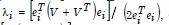 as V was precisely scalable to satisfy We employed Pearson’s correlation coefficient in PySAL for summarizing the autocovariance terms, which were quantifiable between the interpolated, county-level, capture point, signatured, stratified estimator determinants. We defined the covariance of the georeferenced, autocorrelated estimator determinants by dividing the product of the variable standard deviations employing

The formula defined the capture point, time series, dependent, regression correlation coefficients of each autoregressively prognosticated, county-level, zip code stratified, georeferenced, signature capture point, interpolated hot/cold spot in Florida based on the stratified LULC and sociodemographic, estimator determinants sampled. For example, during the validation exercise, we were able to ascertain that many georeferenced eigen-autocorrelated, county, zip code, stratified hot spots of potential leukemia patients were old age retirement facilities throughout the State (Figure 2). The eigenfunction second-order eigen-decomposition temporal filtering approach added a minimally sufficient set of signatured, capture point, georeferenced, stratified, LULC, and sociodemographic, estimator determinant eigenvectors as proxy variables to the set of empirical georeferenced zip code, stratified, county-level, sentinel site, signature capture points. The evidential model prognosticators induced mutual independence in the sampled empirical estimator determinants in eigenvector eigen-geospace. The estimator determinants in scanpy revealed the time series-dependent, predictor variable clustering tendencies at the county zip code level throughout Florida.

The temporal pattern in the eigenvectors exhibited only positive local eigen-autocorrelation and vice versa for negative eigen-autocorrelation. The interpolated, time-sensitive, stratified, hot/cold spot, signature, scalable, autocorrelated, temporal, Gaussian, oncological- related explanators ei and ej within each set of eigenvectors were mutually non-zero, which was revealed using symmetry transformation [i.e.This was expressible employing a quadratic. The quadratic form representation of the eigen-temporal autocorrelation index [i.e., Moran’s I] captured the non-zero autocorrelation in the time series sampled, oncological-related hot/cold spots generated by the authors. The eigen-temporal filtered eigenfunction eigenvectors derived from the georeferenced, stratified, zip code, sampled, hot/cold spot, capture point estimator determinants were eigen-orthogonal but only to the constant unity vector 1 in X. Eigenvectors corresponding to different eigenvalues will be orthogonal if the matrix is symmetric, i.e., real spectral theorem.

The second-order eigenfunction eigen-decomposition allowed linking each collection of the eigenvectors to its specific, georeferenced county, zip code, stratified, sampled capture point, by letting ESAR be a matrix whose vectors were subsets ofA higher-order, stratified, AR, capture point time series model was subsequently constructed in PySAL from the georeferenced, time series, signature, sampled dataset of county, zip code-level stratified interpolated regressors. The model found that the lag orders were mis-specified in the oncological sampled, interpolated time sampled data due to asymptoticness. This violation of the regression assumption in time in the forecasted LULC and sociodemographic, georeferenced, hot/cold spot oncological data we assumed would be a part of the misspecification bias in the asymptotical sampled model estimator determinant dataset, which was subsequently correctly specified using a non-asymptotic order. A non-fixed-effect formula did not remain the same under non-stationarity.

A linearized combination of the non-asymptotical, time-sensitive, regression coefficient subset was approximated by employing the misspecification term of the capture point, interpolated, non-asymptotical, time series, signatured interpolated, LULC, and sociodemographic, estimator determinant model output, which in this experiment was expressible asThe linearized combination ESARγ did not remain eigen-orthogonal to the sampled, non-asymptotical, georeferenced, signatured, time series, dependent, exogeneous variables X and the estimated stratifiable county-level, zip code, hot/cold spot capture points since β ˆ was biased. Furthermore, as a property of the OLS estimator, the approximated term ESARγ was also not eigen-orthogonal to the capture point time series, model residuals εˆ. The model = βˆ + γˆ + εˆ y X ESAR [3.2] eigen-decomposed the georeferenced, non-zero, autocorrelated signature, stratified, capture point, LULC, and sociodemographic,stratified, prognosticated, signatured variables y into a systematic trend component, a stochastic signal component, and white-noise residuals.

The term ESARγˆ removed error variance inflation in the MSE term attributable to potential, latent, time series, heterogeneous erroneous variance embedded in the empirical sampled, georeferenced, zip code stratified, county, aggregation/non-aggregation-oriented, eigen-temporal filtered interpolated, signatured, capture point, non-asymptotical estimator determinants. Subsequently, a temporal lag model was constructed employing ELag which was a matrix of the sampled, estimator determinant eigen-decomposed eigenvectors, which in our forecast oncological model renderings were revealed as a subset ofaTgh.e approximation of any potential misspecification term was subsequently quantifiable employing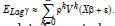Since ELagγ was uncorrelated with the interpolated, county-level, stratified, zip code, signatures, X, its incorporation into the georeferenced, scaled-up, sentinel site, vulnerability- oriented model attempted to correct the temporal bias using estimated plain OLS parameters β ˆ.

The equation y = Xβˆ + ELagγˆ + εˆ [3.3] revealed the specific, empirical sampled, eigen-valued capture point, estimator determinant variance, which were retrievable from the eigen-decomposition of the time lag signatured, LULC, and sociodemographic, stratified, capture point model forecast summary diagnostics. We noted that the trend and the time-series signals were uncorrelated, and the mean square error (MSE) was deflated. The eigen-orthogonal, signatured, eigen-autocorrelated, eigen-spatial filtered, capture point, interpolated model output created multiple, sentinel site, georeferenceable, county-level, zip-code stratified, hot/cold spot, LULC, and sociodemographic, vulnerability-oriented, uncertainty-oriented, probabilistic, signature capture point maps. The misspecification term in each county stratified model was revealed as S(T ) = S(t) exp . The interpretive signature, temporally dependent LULC and sociodemographic capture points, time series, patterns were generated from the prognosticated distribution of the stratified, aggregation/ non-aggregation-oriented, regressed estimator determinants.

There was a requirement to describe independent key dimensions of the underlying uncertainty processes in the empirical sampled oncological time series due to violations of regression assumptions. We were able to define non-asymptotical, temporal estimator determinant patterns in each county zip code model misspecification term. We considered a non-stationary random process x (t ) in the stratified, capture point, time series, prognosticative, interpolated, signatured, oncological-related, model using the Laplace transform. We considered a wide-sense-stationary random process x (t ) . The autocorrelation function was r (t −τ ) := E x (t ) x (τ ) . We let S (s)be the Laplace transform of r (t ) in the oncological-related, forecast, estimator, and determinant model. We computed S (s) as S (s) = E X (s) X (s)∗ , where X (s) was the Laplace transform of x (t ) . We did so to determine if non-asymptotical time series zero or non-zero autocorrelation occurred in the model residuals. In mathematics, the Laplace transform is an integral transform that converts a function of a real variable (usually t, in the time domain) to a function of a complex variable (in the complex frequency domain, also known as the s-domain, or s-plane) [34].

We let S (s) be the Laplace-transform of r (t ) in the forecast, oncological-related, estimator determinant capture point model when S (s) was S (s) = E X (s) X (s)∗ and where X (s)was the Laplace transform of x (t ) . The Laplace transform of R(τ ) was provided by: LR(s) = ∫0 −∞σ 2eατ cos(ωτ )e, , where a non-zero eigen-autocorrelation function was r (t −τ ) := E x (t ) x (τ ) . Our results indicate that the Laplace transform is a powerful tool for analyzing time-domain signals and systems. Laplace transform appears to have potential applications in the field of spatial autocorrelation analysis of time-sensitive, oncological-related, signatured, interpolated, LULC, and sociodemographic, county, zip code stratified, hot and cold spot estimator determinants. A PySAL model output subsequently created multiple, regressively forecastable, county-level, hot/cold spot, Gaussian, zip-code stratifiable, capture point, signature, interpolated, LULC, and sociodemographic, sentinel site maps employing the Laplace transform.

There were no time dependent misspecification terms since S(T ) = S(t) exp .Quantification of the stratified, LULC and sociodemographic, county, zip code stratified, time, series, hot/cold spot capture point patterns were parsimoniously quantifiable from the distribution of the georeferenced, non-asymptotical, non-zero autocorrelated, regressed, aggregation/non-aggregation-oriented, stratified, estimator determinants which in this experiment was a requirement to describe independent key dimensions of the underlying uncertainty-oriented temporal processes in the interpolated capture point, county-level, zip code signatured data throughout Florida. We were able to confirm a non-dependent, linearized, non-misspecified, non-zero, time series pattern in the sampled, capture point regressors. Python provided an efficient interactive tool for organizing and analyzing the stratified, hot/cold spot, non-Gaussian, county, zip code level, signatured interpolated, data capture points.

In the georeferenceable, time-series, dependent, vulnerability- oriented, county, zip code, hot/cold spot, capture point, prognosticative autoregressive modeling, the AR model furnished an alternative specification that was written in terms of a correlation matrix in PySAL. Here, the covariance of the potential, aggregation/ non-aggregation-oriented, time series, stratified, georeferenced, capture point signature data was a function of the matrix (I − ρCD −1 )(I − ρD−1C) = (I − ρWT )(I − ρW), where T denotes the matrix transpose. The resulting matrix was symmetric and was considered a second-order specification, as it included the product of two time-sensitive structure matrices (i.e., WTW). This matrix restricted positive, discrete, integer values of the regressed noisy parameters to the more intuitively interpretable range of 0 ≤ ρˆ ≤ 1. A Python code was subsequently generated for a time-sensitive autoregressive signature model, which was robustly trained using statsmodels. tsa.ar_model.

Euclidean distances between the capture point, temporal, scaled-up, county, zip code, aggregation/non-aggregation-oriented, stratified LULC, and sociodemographic, estimator determinantswere definable in terms of an n-by-n geographic weights matrix, C, whose cij values were 1 if the sampled geolocations i and j were deemed nearby, and 0 otherwise. Adjusting this matrix by dividing each row entry by its row sum subsequently rendered C1, where 1 was an n-by-1 vector of ones, which converted the regression-based matrix to matrix W [i.e., time correlation grid]. The resulting autoregressive signature model specification with no sampled, scaled-up, signatured, interpolated, capture point, stratified, estimator determinants (i.e., the pure autoregression specification) subsequently took on the following form: Y = μ(1 − ρ)1 + ρWY +wεh,ere μ was the scalar conditional mean of Y, and ε was an n-by-1 error vector whose LULC or sociodemographic parameters were statistically independent “normalized” random variates.

Temporal signature, capture point autoregressive models are fit using empirical datasets that contain observations on geographical areas or on any units with a spatial representation. Approximate standard errors for the stratifiable, county, zip code-level, prognosticative, capture point, estimator determinant model was computable as the square roots of the diagonal elements of the estimated covariance matrix. The covariance matrix for analyzing the signature, oncological-related, related capture point, time series, stratified estimator determinants was expressible employing E[(Y − μ1)′(Y − μ1)] = Σ = [(I − ρW′)(I − ρW)]−1σ2, where E(•) designated the calculus of expectations, I was the n-by-n identity matrix denoting the matrix transpose operation, and σ2 was the error variance. The variance of the non-homogeneous, prognosticated, aggregation/ non-aggregation-oriented, signatured, georeferenced, LULC and sociodemographic, capture point, estimator determinants were spread out temporally.

We introduced the conditional variance at time t of the log-return yt (of a georeferenced, interpolated, zip code stratified, capture point denoted by ht , which was postulated to be a linearizable function of the squares of past q log-returns and past p conditional variances in the GARCH model. More precisely: ht =α 0 + Σi =1qαiyt − i2 + Σ j =1pβ jht − j, where the capture point zip code, oncological-related, LULC, or sociodemographic, stratified time series parameters satisfied the constraints αi ≥ 0(i = 0,...., q) and β j ≥ 0( j =1,...., p) in order to ensure a positive conditional variance. It turned out that the simple specification p = q =1 was able to reproduce the forecastable volatility dynamics of the sentinel site, signatured, data capture points. This led the GARCH (1,1) model to tease out the time erroneous prognosticative non-Gaussian, interpolated variables. Given a model specification for ht , the log-return was then modelled as yt =ε tht1/ 2 , where ε t were the i.i.d. disturbances.

The student-t specification was particularly useful, since it provided the excess kurtosis in the conditional distribution found in the time series oncological-related, signature capture point interpolated processes (unlike models with Normal innovations like those contributed to the literature). Until recently, eigen Bayesian, GARCH, semiparametric, non-frequentist models have mainly been estimated using the classical Maximum Likelihood technique. Our formulation approach generated an attractive alternative which enabled time series robustification of the georeferenceable, capture point hot/cold spot, signatured, estimation, zip code model stratification with probabilistic statements on time series asymptotical heteroscedastic functions embedded in the model parameters. We employed truncated normal priors on the non-frequent, Markovian semi parameterized, GARCH renderings where α and

β p (α )αφ N2(α |μα ,Σα )1{α ∈R + 2} p(β )αφ N1(β |μβ , Σβ )1{β ∈R +}

and where μ ⋅ and Σ⋅ were the hyperparameters. In this experiment, 1{⋅} was the indicator function and φ Nd was the d-dimensional normal density.

The prior distribution of vector ϖ conditional on ν was found by noting that the components ϖ t were i.d.d from the inverted gamma density, which yielded

Quantifying the prior density was useful in this experiment for two reasons. First, it was potentially important for numerical reasons to bound the degrees of freedom in the stratified, georeferenced, capture point, time series, sampled, signature interpolated, capture point, LULC, and sociodemographic stratified parameters to avoid an explosion of the conditional variance. Second, we approximated the normality of the time-sensitive errors while maintaining a reasonably tight prior, which improved the convergence of the sampler. We let Fs denote the information set generated by {Xk; k ≤ s} , namely, the sigma field σ ( Xk; k ≤ s It was easy to see that Fs was independent of ε t for any s < t . According to the properties of the conditional mathematical expectation in the county, zip code stratifiable, oncological-related forecast vulnerability model.

We achieved E ( Xt | Ft −1) = E (σ tε t | Ft −1) =σ tE (ε t | Ft −1) =σ tE (ε t ) = 0 and

Var ( Xt2 | Ft −1) = E ( Xt2 | Ft −1) = E (σ t2ε t2 | Ft −1) =σ t2E (ε t2 | Ft −1) =σ t2E(ε t2) =σ

This implied that σt2 was the conditional variance of Xt, and it evolved according to the previous georeferenced, zip code stratifiable, hot/cold spot eigen-sampled interpolated, capture point signature values of {Xk2;t − p ≤ k ≤ t −1} . We subsequently considered the ARCH (1) model {Xt =σ tε tσ t2 =ω +α1Xt −12 Explicitly, the unconditional mean was quantifiable employing E ( Xt ) = E (σ tε t ) = E (σ t ) E (ε t ) = 0 in the oncological model. Additionally, the ARCH (1) signature capture point, time series was expressible as

Xt2 =σ t2 + Xt2 −σ t2 =ω +α1Xt −12 +σ t2ε t2 −σ t2 =ω +α1Xt2 +η . That is,

Xt2 =ω +α1Xt2 +ηt where ηt =σ t2(ε t2 −1) . It was shown that ηt is a new white noise generated from non-homoscedastic, non-Gaussian time series data, which were the stratified estimator determinants. In this experiment, the model residuals were quantifiable if 0 <α1<1. Eq. (2.4) was a stationary AR (1) model for the series Xt2 . Thus, the unconditional variance

Var ( Xt ) = E ( Xt2) = E[ω +α1Xt −12 +ηt] =ω +α1E ( Xt2)

was then transformed to Var ( Xt ) = E ( Xt2) =ω1−α1. Moreover, for h > 0 , the time-dependent non-Gaussian estimator determinant properties of the conditional mathematical expectation, and by equation (2.4), then generated

E ( Xt + hXt ) = E (E ( Xt + hXt | Ft + h −1)) = E ( XtE ( Xt + h | Ft + h −1)) = 0 .

The final mathematical representation of the oncological-related, eigen Bayesian semiparametric, non-frequentist capture point, scaled-up, Markovian, prognosticative, signatured county, zip code, stratified GARCH/ARCH model formulation was describable as:

e. p was the order of the eigen-Bayesian semiparametric Markovian GARCH terms, and

f. q was the order of the eigen-Bayesian semiparametric Markovian ARCH terms.

The eigen-Bayesian semiparametric Markovian GARCH (1,1) model (one ARCH term and one GARCH term) employed the specification: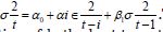

This formulation allowed for quantification of both short-term time non-Gaussian shocks and long-term volatility persistence due to violations of regression assumptions in time in the model capture point sampled estimator determinants. In this equation, 0 β was composed of estimator determinants presenting the reference category of each variable 1...m. x The semiparametric eigen-Bayesian, Markovian, capture point probability model was constructed based on the probability of a binary label [ zero or non-zero time series autocorrelation] given a feature vector:

model and its variants were subsequently employed to model and correct for geo-spatiotemporal latent multicollinearity and other non-Gaussian components due to violations of the regression assumption in time. The georeferenced empirical dataset of scaledup, capture point, sentinel site, prognosticative, capture point, semi-parameterizable, oncological-related, estimator determinant, eigen-Bayesian semiparametric Markovian GARCH (1,1) ARCH model with autoregressive dependent errors was illustrative as follows;

This model combined the mth-order autoregressive error model with the eigen-Bayesian semiparametric Markovian GARCH (1,1) /ARCH ( p, q) variance model. The paradigm was denotable as the AR(M ) -GARCH( p, q) regression model. The tests for the presence of ARCH effects (namely, Q and LM tests, from Lee and King and from [35] helped determine the order of the signature, interpolated, capture point, eigen-Bayesian, semiparametric, Markovian, Gaussian, estimator determinants, which was appropriate for the aggregation/ non-aggregation-oriented county-level, zip code, stratified oncological -related, LULC and sociodemographic, interpolated time series data. For example, the LM tests examined here were significant ( p < 0.0001) , which indicated that a very high-order model [i.e., eigen-Bayesian semiparametric Markovian GARCH (1,1) / ARCH] was needed to model the asymptotical, time-heteroscedastic, scalable, signatured, county-level, zip code georeferenceable, stratifiable capture points.

The oncological-related, forecast, signature, capture point, eigen-Bayesian semiparametric Markovian GARCH (1,1) /ARCH model quantified the erroneous time series data and described the variance of the uncertainty misspecification term or innovation, as a function of the actual sizes of the previous time periods’ error terms. We noted that the variance was related to the squares of the previous innovations. When the potential eigenized, time series dependent, scaled-up, county-level, stratified, georeferenced, zip code, signatured, prognosticated, estimator determinant, data capture points were used in the eigen-Bayesian semiparametric Markovian GARCH (1,1) /ARCH analysis, the error term was not independent through time. Here, the errors in the capture point, sentinel site oncological-related, prognosticative model were diagnosed as serially temporally correlated. If the error term is autocorrelated, the efficiency of OLS parameter estimates is adversely affected, and standard error estimates are biased.

The county-level, stratified, signatured, zip code, capture point, estimator determinant model did not require the approximation of many time lag coefficients. The eigen-Bayesian semiparametric Markovian GARCH (1,1) /ARCH model improved the time series, oncological-related capture point sampled, and estimator determinants by replacing assumptions of constant volatility with conditional volatility (Table 1-8). The presence of ARCH effects in the return series was confirmed by the ARCH LM-test (χ² = 355.9, df = 12, p < 0.001), justifying the use of GARCH modeling. Post-estimation diagnostic tests on the standardized residuals showed no remaining ARCH effects (χ² = 3.461, df = 12, p = 0.991), indicating that the GARCH (1,1) model successfully captured the conditional heteroscedasticity in the data. In our prognosticative, capture point vulnerability- oriented, county-level, oncological-related, eigen-Bayesian semiparametric Markovian GARCH (1,1) /ARCH model, the conditional temporal heteroscedasticity portion was that volatility in the paradigm was nonconstant. Substituting this transformation employing the empirical, time-sampled, aggregation/non-aggregation- oriented, stratified, sampled, sociodemographic, and LULC eigen-geospatially filtered estimator determinants rendered:

Table 1: Conditional Variance Dynamics.

Table 2: Pre-ARCH LM-test.

Table 3: Optimal Parameters.

Table 4: Robust Standard Errors.

Table 5: LogLikelihood & Information Criteria.

Table 6: Box-Ljung Test on Standardized Residuals.

Table 7: Box-Ljung Test on Squared Standardized Residuals.

Table 8: ARCH LM-Test on Standardized Residuals.

Consequently, the stratified, geosampled, capture point, county-level, georeferenceable, zip code, hot/cold spot, signatured, estimator determinants obtained employing the new time-series, dependent, prognosticative Gaussian variables were correlated with the misspecification term. Under this condition, standard OLS results for the basic regression model y = Xβ + ε∗ generated from the signature estimator determinants provided time-biased estimates β ˆ of the underlying regression parameters β.

The correlation, or lack thereof, between the georeferenced, temporal heteroscedastic, non-Gaussian, stratified, aggregation/ non-aggregation-oriented, georeferenceable, LULC and sociodemographic, prognosticative signatured, capture point variables and the misspecification terms in the scaled-up, autoregressive, oncological- related, forecast, eigen-Bayesian, semiparametric, Markovian GARCH (1,1) /ARCH model were employed to design spatial proxy variables so the non-Gaussian properties of the model due to violations of regression assumptions in time could be satisfied. Misspecification of the main exposure capture point variable and other stratifiable county, zip code LULC, and sociodemographic, estimator determinants may not be uncommon in time–series, dependent, multivariate, estimator determinant, oncological-related time series, sampled, county-level, vulnerability regression models. A dataset of eigen-decomposed, Bayesian, Markovian, non-frequentist semi-parameterized eigen-orthogonal eigenvalues was generated, which were equal to coefficients of the quantified time-sensitive eigen-autocorrelated variables post-multiplied by a constant.

Eigenvectors associated with high positive (or negative) eigenvalues have high positive (or negative) autocorrelation. The diagonalization of the eigen-Bayesian, autocovariance, uncertainty- oriented correlation matrix generated from the sampled, time weighted, oncological-related estimator determinant, capture point stratified data consisted of quantitating the normalized vectors u i , stored as columns in the matrixU = u u , satisfying:

terminants were centered, and at least one eigenvalue was equal to zero when

(3.5) Considering the centered vector z = Hx and using the properties of idempotence of H, equation (3.5) was equivalent to:

(3.6). As the temporally sensitive capture point eigenvectors u i and the vector z were centered, equation (3.6) was rewritten as:

The distribution of the temporal regressed, eigen-Bayesian semiparametric Markovian GARCH (1,1) /ARCH, capture point model residuals in the autocovariance matrix was then quantified. The maximum value of I was obtainable by the variation of z, as explained by the temporal semi-parameterized eigenvector 1 u , which corresponded to the highest eigenvalue 1 λ in the time series, nonfrequentist, regression-related prognosticative model. We used the Inverse negative Hessian (INH), i.e., (−H ) ^ −1, for optimization and statistical inference of the sampled stratified, georeferenced, capture points. Oncological-related time series, LULC, and sociodemographic interpolated the estimator determinants robustly since we were dealing with MLE. We interpreted this product as an approximation of the covariance matrix of the scalable, county, zip code, and oncological-related parameters. Specifically, when maximizing a likelihood function, the inverse of the negative Hessian (or the negative of the Hessian, which is the observed Fisher information) provides an estimate of the variance-covariance matrix of the estimated parameters.

dardized time distribution was the estimable number of degrees of freedom (vv) . We let Ht denote the capture point, county, georeferenced, zip code, signatured, sociodemographic, and LULC sample frames available at time t, t = 1, ..., N . The likelihood function for the innovation series was provided by

where f was a standardizable Gaussian t density function. The exact form of the loglikelihood objective function depended on the parametric form of the innovation distribution. Since our t z had a standard Gaussian distribution, the loglikelihood function in the eigen-Bayesian, semi-parametric, Markovian, non-frequentist, signature, capture point, time series model was

We found that our eigen-Bayesian. semiparametric, time series, dependent, GARCH/ARCH eigen-autocorrelation approach was more adaptable to an exploratory specification search of the relevant scalable, georeferenceable, sentinel site, oncological stratified, capture points at the county, zip code level for [i.e., aggregation of potential patient households]. In contrast, for the simultaneous autoregressive model, the eigenvectors {e1, , en}SAR rendered from the eigen-Bayesian forecast model employed the projection of M(X ) on the approximated sentinel site, sampled capture point, time series variables X. Thus, any change in the underlying model structure required a recalculation of the eigen temporal filters for generating robust tessellations. Eigen Bayesian, semi-parametric temporal filtering of either the lag model or the simultaneous autoregressive model with a common factor constraint, thereafter, only required identification of one set of selected time-sensitive eigenvectors, namely, ESAR or ELag , respectively.

The relevant set of eigenvectors was applied simultaneously to the georeferenced, multivariate, capture point, sentinel site, scaled-up, aggregation/non-aggregation-oriented, signatured, hot/ cold spot, stratified, zip code, oncological estimator determinants. For the generic autoregressive model, eigen-spatial filtering was applied individually to each sampled, aggregation/non-aggregation- oriented, eigenized, time series, sampled estimator determinants. The generic specification of autoregressive models associated a specific time lag factor with the y variable and other lag factors for each additional, operationalizable, aggregation/non-aggregation- oriented, oncological-related, time-series specified, estimator determinant. The eigenvectors {e1, , en}Lag filtered latent zero, temporal, eigen-autocorrelation erroneous non-Gaussian coefficients embedded in the generic, scaled-up, prognosticative, capture point, interpolated risk model for each georeferenced, aggregation/ non-aggregation-oriented, sentinel site, semi-parameterized, sociodemographic, and or LULC, stratified non-frequentistic georeferenced, county, zip code-level sampled estimator determinant.

Discussion

This paper contributes to the analysis, interpretation, and use of an eigen-Bayesian, semiparametric, non-frequentist, Markovian GARCH/ARCH model formulation, utilizing correlated oncological- related, stratifiable, county, zip code, signature, interpolated, capture points, and sampled time-series estimator determinants. The effect of ignoring the time non-Gaussian correlation structures of the regression process is investigated. The results reveal a spurious impact of the time correlation on the eigenvalues in the predictive oncological model. To mitigate this impact, a post-eigen filtering procedure to whiten the data is applied. We assumed that by identifying and rectifying heteroscedastic and multicollinear signatured, interpolated, LULC, and or sociodemographic time series, residual, zero autocorrelated, non-Gaussian estimator determinants, we would be able to generate a robust social messaging platform precisely targeting oncological-related patients at the county zip code level in Florida using an AI-ML infused smartphone interactive app.

Initially, for the empirical sampled, time series, georeferenced, signature, interpolation mapping the county, zip code level, scalable, georeferenced, oncological-related capture points [i.e., Sampled LULC and sociodemographic, estimator determinants of potential leukemia patients with a household of $487,000 value in zip code 33647 in Hillsborough County, Florida, we employed subject-specific time series dependent hot and cold spot, stratified, estimator determinants which were scaled-up using a non-bilinear, non-stochastic, interpolator. Non-stochastic interpolation refers to deterministic interpolation methods, which can estimate geospatially forecasted capture point signature values at unmeasured locations based on the surrounding measured values. Unlike geostatistical methods (e.g., Kriging), which rely on pre-determined spatial contexts like the degree of similarity or smoothing, our non-bilinear, non-stochastic interpolator attempted to noiselessly scale-up and non-zero eigen-autocorrelated potential, non-Gaussian, temporally erroneous dependence, and non-homogeneous variance between the empirical sampled, georeferenced, county-level, zip code, stratified, capture point, signatured, stratified estimator determinants.

We employed the Spatial Autocorrelation (Global Moran’s I) tool in PySAL to measure latent zero non-Gaussian eigen-autocorrelation coefficients in the empirical, georeferenced, interpolated, capture point, oncological sampled, LULC, and sociodemographic, estimator determinant dataset. Using a set of georeferenceable, time series dependent, county, zip code, stratifiable, oncological-related data, capture point, feature attributes, we evaluated whether synthetic eigen-decomposed, eigenvectors derived from time series weighted, aggregation/non-aggregation-oriented, interpolated patterns were clustered, dispersed, or random. Here, the tool in PySAL calculated the Moran’s I value and a z-score (i.e., standard deviations) and p-value to evaluate the significance of the georeferenced hot/cold spot, stratified, time series estimator determinants. P-values revealed the numerical approximations of the county, zip code, and capture point regression distribution. Our capture point forecast model revealed non-zero, Gaussian, time series autocorrelation. PySAL provided an efficient interactive tool for organizing and analyzing the stratified, time series, dependent, georeferenced, eigen-decomposed, non-zero autocorrelated, hot/cold spot capture points.

of the intercorrelation function Rxy (k ) in the model forecasts. In so doing, we were able to demonstrate that Sxy (z) = Syx (z −1) . The correct expression then was quantifiable as

The expression converted every oncological-related, stratified, georeferenced, county, zip code, Z-transform, estimator, determinant time signal by a sequence of eigen-decomposed, county-level, sentinel site capture points. These sentinel sites were subsequently transformed into a complex frequency domain representation. We considered this product as a discrete-time equivalent of the Laplace transform. The Laplace transform is an integral transform that converts a function of a real variable ( tin the time domain) to a function of a complex variable s (in the complex-valued frequency domain, also known as the s-domain, or s-plane [36]. In this experiment, the Laplace transform was used to solve differential equations, particularly those involving linear time-invariant systems, by converting them into algebraic equations. The Laplace transform simplified the process of finding solutions by analyzing the time behavior and stability of the oncological model based on the interpolated LULC and sociodemographic time series sampled, signature stratified data. The Laplace transform provided a lot of insight into the nature of the model equations by converting between the time and the frequency domains.

We obtained robust non-stationary, stratifiable, georeferenceable, oncological-related, empirical time series, sampled, capture point, non-Gaussian, estimator determinants of the time noise in the oncological model residuals. We obtained a higher degree of spectral Gaussian flatness by using an adaptive pre-whitening filter. This filter was based on supervised noise [i.e., Wiener-Kolmogorov]. We employed the Wiener-Kolmogorov whitening procedure, which decomposed the Laplace transform of R(τ ) into the product of white noise and a system function (s) =W (s)H (−s)H (s) in Python. Then letting h(t ) = L −1(H (s)) and

w(t ) = L −1(W (s)) the time series, sampled, county, zip code, oncological data was given by: dhdt = f (h,t )h(t ) + w(t ) where f (h,t ) which was a function that satisfied dhdt = f (h,t )h(t ). The Wiener-Kolmogorov filter is an optimal prediction of the stratified, county, zip code time series, which relies on minimizing the mean square error (MSE) between the filtered output and a time signal. This optimization process involved calculus and the use of partial derivatives.

The partial derivatives of all the functions with respect to the georeferenced, county, zip code level, oncological-related, stratifiable, hot/cold spot, county, zip code, time series, capture point, and signature interpolated observational prognosticators revealed violations of the regression assumption in time. x1, , xn was organized in an m-by-n matrix,

that can quantify time derivatives. The Jacobian matrix described how the empirical sampled signature interpolated LULC and sociodemographic estimator determinants changed with respect to its input variables at a stratified, county, zip code, specific hot or cold spots in time. The matrix captured the local, instantaneous response to time perturbations around a steady state. The eigenvalues of the Jacobian matrix revealed information about the model’s final stability. For instance, since all eigenvalues had negative and positive real Gaussian non-zero autocovariance, the model residuals were stable.

Time eigen-autocorrelation revealed different lags at one capture point in time, which was then related to values at a later capture point in time, thereby capturing the dependencies in the oncological sampled, hot/cold spot, stratified estimator determinants. In the context of spatial modeling, particularly in empirical time series, stratifiable, georeferenceable data capture point models, the Hessian matrix can be applied to derive the non-asymptotic distributions of regression coefficient estimates. In this experiment, the inverse of the Hessian matrix from optim() was employed as the non-asymptotic covariance matrix for estimating the non-Gaussian time series parameters. Here, the non-asymptotic covariance matrix was an approximation of the covariance matrix of the sampling distribution. The matrix was significant in the statistical analysis as it provided insights into the variability of the signature, capture point, oncological-related, time series, sensitive, estimator determinants. The Hessian matrix helped evaluate the reliability and precision of the interpolated signatured, capture point, georeferenced, non-zero autocorrelated, county, stratified, zip code, hot/cold spot, estimator determinants obtained from the regressively forecasted, uncertainty-oriented oncological model.

The forecasts from the matrix accounted for non-zero, non-asymptotic, Gaussian, eigen-filtered temporal eigen-autocorrelation. When analyzing scalable, oncological-related, stratifiable capture points with eigen-time autocorrelation, especially within complex eigen-spatial oncological prognosticative signature interpolated models, the Hessian non-asymptotic covariance matrix can contribute to understanding the statistical erroneous time-sensitive properties and the validity of an empirical interpolated dataset. Non-Gaussian asymptotical, prognosticative, capture point, county, zip code stratifiable, signatured, time series sampled, and interpolated estimator determinants were generated in a Jacobian matrix. Most of the contributions to the literature to date proposes approximations to the determinant of a positive definite n × n spatial covariance matrix (the Jacobian term) for Gaussian spatial autoregressive models that fail to support the analysis of massive time series, sampled, oncological-related, county-level, zip code, stratifiable, empirical georeferenced datasets, In vector calculus, the Jacobian matrix of a vector-valued function of several variables is the matrix of all its first-order partial derivatives.

Here, the Jacobian approximations selected eigen decomposed eigenvalue estimation techniques, summarized validation results for the estimator determinant capture point eigenvalues, and facilitated non-zero eigen-autocorrelated parameters. The Jacobian determinants at a given capture point provided important information about the behavior of a sampled oncological-related estimator determinant in time near a county zip code hot spot stratified capture point. For instance, the continuously differentiable function f was invertible near a capture point [ p∈Rn] if the Jacobian determinant at p was non-zero. [i.e., inverse function theorem] [37]. In real-time data analysis, a branch of mathematics, the inverse function theorem is a theorem that asserts that, if a real function f has a continuous derivative near a capture point where its derivative is nonzero, then, near this point, f has an inverse function [38-44]. The theorem applies verbatim to complex-valued functions of a complex variable (example: a time series coefficient in a leukemia model). Here, the inverse function rule expresses its derivative as the multiplicative inverse of the derivative of f .

It generalized to functions from n-tuples (of the oncological time series estimator determinants) to functions between vector spaces of the same finite dimension, by replacing “derivative” with “Jacobian matrix” and “nonzero derivative” with “nonzero Jacobian determinant”. The principal contribution of this paper was to aid in the implementation of the time-sensitive, autoregressive, prognosticative model, signature interpolated, capture point, non-noisy time series specifications for the georeferenced oncological-related, empirical estimator determinants. Our specific eigen-autocorrelation additions to the predictive vulnerability oncological modelling literature include (1) new, more efficient capture point signature interpolation uncertainty estimation second order eigen-algorithm; (2) an approximation of the Jacobian term for sampled census and landscape data forming complete state, county and zip code regional coverage; (3) issues of interpolated estimator determinant inference from a county, zip code stratified, scaled-up capture point; and (4) rectification of non-Gaussian hot/cold spot causation covariates due to violations of regression assumptions in time.

For the fixed, georeferenced, county, zip code, stratified capture point, scaled-up, oncological-related interpolated time series parameters, a suitable choice was the diffuse prior (i.e., p(γ) const., but a weakly informative Gaussian prior was also possible). A second-order Gaussian random walk prior can allow sufficient flexibility while penalizing abrupt changes in time-sensitive regression functions in a county, zip code, oncological-related, predictive, signature, or capture point model. The second-order random walk model may be suitable for smoothing empirical samples, georeferenceable, oncological capture point estimator determinants, for quantifying response functions that here reveal a transitionary, non-Gaussian, temporally rectified, non-zero, autocorrelated signature interpolated covariates computationally using the Markovian properties of the joint (intrinsic) Gaussian density. From the time series autocorrelation plot generated, it was apparent that less of the upper tail in the oncological-related forecast model was included around the highest posterior density in the quantile-based probability time interval due to the non-stochastically interpolated, capture point, zip code, signatured, LULC, and sociodemographic, stratified estimator determinants. The high probability distribution (HPD) interval does not produce equal tails when inappropriate.

However, both the quantile-based probability interval and HPD interval in the capture point oncological model forecasts did take the prior distribution into account [i.e., potential, scaled-up, county-level, georeferenceable, aggregation/non-aggregation, time series, empirical sampled, non-zero, autocorrelatable, time series estimator determinants]. These intervals represented the analogue of CIs in the model. Appealing properties of eigen-decomposed capture point, time sensitive, county, zip code stratifiable, georeferenced, oncological-related eigenvectors include: (1) they are mutually orthogonal and uncorrelated; (2) a single eigenvector is proportional to the vector 1, the intercept covariate in a regression model; and, (3) eigenvectors are usable to temporally visualize, the full spectrum of possible degrees of non-Gaussian, zero, eigen- autocorrelation in an empirical sampled dataset of georeferenceable, county, zip code, stratifiable, oncological-related capture points and their sampled estimator determinants. PySAL conducted the invasive geospatial time series eigen-autocorrelation signature residual forecast analysis, for further detection of erroneous clusters, [i.e., sociodemographic, stratified, time series, hot spots] and non-clustered LULCs [i.e., cold spots] at the county level, stratified, county, zip code, locations based on outlier graphs constructed using the stratified, capture point interpolated signatures.

Temporal eigen-filters are usable to decompose a Jacobian matrix into a georeferenced signature, empirical dataset of capture point, oncological-related, time series stratified eigenvectors and eigenvalues, which are applicable to determine non-Gaussian time series dependent regressors in an oncological-related, prognosticative, vulnerability-oriented, signature interpolation model. The eigenfunction eigen-decomposed, capture point, estimator determinant oncological-related, signature interpolation model optimized predictively targeting and prioritizing, georeferenceable, county level, zip code hot/cold spot locations by generating non-asymptotical stratifiable, non-zero non-Gaussian, autocorrelated, estimator determinants temporally. Our eigenfunction signature eigen decomposition is appropriate when a contiguous region on the right or left (or both) of the input is expected to deviate systematically in a time series, sensitive, county, zip code level stratifiable, predictive risk model. Such regions (i.e., potential non-asymptotic regions) did not occur in the vulnerability-oriented, dependent, capture point, vulnerability-oriented prognosticative model analysis in as the data were non-time series.

Here, the local temporal non-asymptotic normality property was quantifiable for the LULC and sociodemographic stratified, signature model estimator determinants for heuristically optimizing targeting and prioritizing, predictive oncological-related county, zip code, hot/cold spot capture point, and interpolated signatures temporally. An eGARCH was subsequently constructed for quantifying temporal heteroscedasticity in the stratified interpolated, county, signatured, zip code, georeferenced, LULC, and sociodemographic, capture point, estimator determinants based on the non-homogeneous gamma distributed mean. The eGARCH model revealed the non-constant error variance over time, including a non-Gaussian prior based on the volatility quantified temporal uncertainty in the non-stochastically interpolated capture point signatures. This model checked the temporal monotonic assumptions in the sample georeferenced county, zip code estimator determinant, signature, capture point, hot/cold spot empirical dataset prior to computing the interpolated heteroscedastic coefficients due to violations of regression assumptions in time. The influence of unequal variance with time in the scaled-up volatility model generated potentially high standard deviations, followed by a high variance due to extreme outliers.

These data violated the time monotonic assumptions in the correlation matrix by distorting its ranking due to the high and low volatility variance flux in the oncological-related interpolated signature estimator determinant model, capture point, and empirical sampled dataset. The model rendered robust results by deflating the p-values, type I and type II errors due to regression assumption violations over time. Moreover, smoothing out the extreme time series outliers in the signature, capture point, eGARCH model accurately represented the monotonic relationships in the correlation matrix without bias due to high kurtosis and skewness. Hence, the output of the interpolated, georeferenced, empirical sampled dataset precisely captured the onset and termination period of the stratified, capture point, time series, signature LULC and sociodemographic, estimator determinants. This was crucial for understanding the temporal disturbances in the zip code, time-sensitive signature, and interpolated hot/cold spots locations at the county level throughout Florida. The fine eGARCH model was a generalizable hierarchical uncertainty model that captured time volatility clustering by modeling the previous squared error terms and current variance over time. We developed an extension of the eGARCH model, the ARCH model.

The ARCH model was a non-generalizable model that captured the past squared error terms [i.e., temporal shocks], which was primarily focused on the time series, volatility signature, interpolated,capture point, oncological, and sampled estimator determinants. The scaled-up, capture point ARCH model was more stable and provided better flexibility than the eGARCH model for capturing long-term conditional residual temporal heteroscedasticity in the time series sampled, oncological-related estimator determinants due to the inclusion of its lagged variances. An exponential function was applied to the interpolated, zip code, stratified, georeferenced, time signatured, capture point, LULC, and sociodemographic, county sampled data to detect temporal erroneous fluctuation patterns, such as leptokurtic and platykurtic tails, incorporating outliers (non-Gaussian latent zero autocovariance). The lag order was quantifiable based on the significant results of the Autocorrelation Function (ACF), Partial Autocorrelation Function (PACF), Akaike Information Criterion (AIC), and Bayesian Information Criterion (BIC). Moreover, the non-significant p-value of the post-ARCH-LM, Ljung box test, and chi-square statistics were considered to validate the stratified, county, zip code, capture point, time series, empirical sampled, oncological-related, signature, model estimator determinants.

This study tested the signature estimator determinant distributions to quantify non-constant temporal error variance based on extreme skewness, kurtosis, and leptokurtic/platykurtic tails in the oncological estimator determinants. These distributions tested Gaussian, Student’s t, and Generalized Error Distribution (GED) in the sampled estimator determinant empirical datasets. In addition, the skewed component was added to the student’s t and GED priors, involving degrees of freedom, mu, and rho parameters to incorporate the heavy skewness and kurtosis in the time series sampled, capture point, heteroscedastic signatured empirical capture point dataset. These priors had the ability to incorporate extreme outliers on the leptokurtic and platykurtic tails, thereby encompassing the extreme events, like potential, georeferenceable, oncological-related, county-level, zip code stratifiable, capture-point hot/cold spots for an accurate understanding of the regression error dynamics in time. The most optimal georeferenceable, stratifiable, interpolated LULC and sociodemographic, estimator determinant distribution subsequently captured latent temporal, multicollinearity involving all the variable dependencies and the goodness of fit criteria in the non-asymptotical oncological model. We employed an eigen-temporal filtered, MCMC simulation procedure for fitting the sampled, county-level, scaled-up, inferential, time series, dependent, estimator determinants. In probability theory and statistics, a Markov chain is a stochastic process that satisfies the Markovian property (usually characterized as “memory lessness”) [www.mathworld. wolfram.com].

We assumed an empirical, sampled, interpolated, LULC and sociodemographic, signature, stratified, capture point estimator determinant empirical dataset of sampled, non-zero, eigen-autocorrelated, county-level, zip code stratifiable, oncological model forecasts [i.e., eigen decomposed, aggregation/non-aggregation- oriented, non-multicollinear, non-heteroscedastic estimator determinants] could account for any non-asymptotical, multivariate geo-spatiotemporal bias in a simulated, interpolated, signatured, capture point Markovian, semiparametric, eigen-Bayesian model output. In so doing, we assumed we would also be able to quantify conditional, autoregressive temporal non-Gaussian sensitive perturbations in eigenvector eigen-geospace due to violations of regression assumptions in time. We found that an empirical, signatured eigen-algorithmic, non-homogeneous, eigen-filtered, georeferenced empirical sampled dataset of eigen-autocorrelated time series stratified, LULC, and sociodemographic, zip code signature interpolated, capture point estimator determinants, could optimally forecast and delineate potential interventional, study site, hot/ cold spot zip code geolocations (e.g., old age community center sentinel sites) in Florida precisely; remote validation revealed diagnostic sensitivity and specificity statistics approaching 100 %. Subsequently, we estimated the eigen-Bayesian semiparametric non-Gaussian residual components in the eigen-autocorrelation oncological-related, capture point model by employing the forecasts from the interpolator.

By invasively examining the non-asymptotic rates, we revealed the consistency and efficiency of the time series, sampled, capture point, regressed county, zip code level, georeferenced hot/cold spot, estimator determinants, and their erroneousness in the absence of prior knowledge. Even a cursory look at the stratified, time series dependent, interpolated, hot/cold spot, signatured, capture point data suggested that some county zip code hot spots geolocations were riskier than others. We noted that the expected value of the magnitude of error terms at times was greater than at others based on scaled-up, time-signatured, capture points. Moreover, these risks were not scattered randomly across quarterly or annual time series, dependent, county-level, sociodemographic, and LULC, interpolated, zip code, stratified data capture points. Instead, there was a potential degree of zero autocorrelation in the riskiness of the model forecasts [i.e., falsely forecasted zip code level, locations of stratifiable, georeferenceable, capture point, hot/cold spots]. Using comprehensive simulations, we demonstrated the finite sample performance of our method, which corroborated the theoretical findings of the ARCH. The ARCH models dealt with a set of noisy temporal issues related to the georeferenced, signature-interpolated oncological stratified covariates.

The model residuals provided a temporal volatility measure for precise forecast mapping, stratifiable, county-level, georeferenceable zip code, hot/cold spots of potential oncological-related patients for intervention [e.g., implementing a prevention leukemia protocol at a senior citizen assisted county treatment facility]. The ARCH model allowed the interpolated, capture point, signature. LULC/sociodemographic, stratified, time series weights to be estimated accurately, i.e., temporally homoscedastically. The non-multicollinear model output allowed the predictors to determine the best weights for optimally forecasting the variance. ARCH models may be employable to describe a changing, possibly volatile variance in an empirical dataset of georeferenced signature interpolated LULC and sociodemographic, explanatory, time series, sampled estimator determinants associated with oncological processes. Although an ARCH model could be used to describe a gradually increasing variance over time, it may be employable in forecast modelling situations in which there may be short periods of increasedvariation in non-stochastically interpolated, LULC, and sociodemographic, signatured, capture point, sampled, oncological-related, time series estimator determinants.

Gradually increasing variance connected to a gradually increasing mean level in an empirical sampled, county, georeferenced, interpolated zip code, stratifiable LULC/ sociodemographic signature model might be better handled by transforming the time variable pre and post ARCH model. The generalization of the GARCH/ARCH parameterization allowed the usage of a weighted average of the past squared signatured oncological-related, capture point residuals quantitated from the georeferenced, interpolated time series, estimator determinants, but it had declining weights which never achieved zero. The models generated forecasts [i.e., precise locations of georeferenced counties, zip code level, stratifiable, hot and cold spots] which were mappable in their simplest form in Python. The GARCH /ARCH specification asserted that the optimal predictor of the variance in the following sample time period employing the weighted average of the long run average variance, the variance predicted for a period, and the new information for a present period was the most recent squared residuals in the signature stratified, prognosticative, vulnerability, county-level zip code model. The model predicted the conditional variances. The summary diagnostics validated the georeferenced specificity and sensitivity based on the forecasts, which also revealed a sensitivity and specificity diagnostic summary output approaching 100 per cent.

Erroneous temporality due to violations of regression assumptions may be quantifiable using an eigen-Bayesian, semi-parametric, non-frequentist, GARCH/ARCH model formulation. For example, if zero time series erroneousness is present in a post-GARCH/ ARCH selected time series, an oncological-related empirical georeferenced dataset of estimator determinants, one would have to conclude the model’s non-Gaussianism is due to time heteroscedastic uncertainty. In an oncological, county, zip code prognosticated capture point, signatured model output, a depreciation in chi-square can be considered a conversion from temporal heteroscedasticity to temporal homoscedasticity. We were able to quantify the violation of regression assumptions in time due to heteroscedasticity using the eigen-Bayesian, semi-parametric, non-frequentist, GARCH/ ARCH model formulation, which modeled the variance of a time series in the estimator determinants. In eigen-Bayesian, semi-parametric non-frequentist, GARCH/ARCH models, an excessively large number of parameters [> 10,000] and the requirement of positive definiteness of the covariance and correlation matrices may pose some difficulties during time series estimation when quantifying stratified, LULC, and sociodemographic, oncological-related, signatured hot and cold spot estimator determinants.

To avoid these issues for future research, we propose two modifications to eigen-Bayesian, semi-parametric, non-frequentist, GARCH/ARCH signature capture point, forecast models. An oncologist or other research collaborator may employ two spherical parameterizations: the Cholesky decompositions of the covariance and correlation matrices. In their full specifications, the introduced Cholesky models may allow for a reduction in the number of stratified capture point, time series sensitive, georeferenced, signatured estimator determinants compared with their traditional non-time series counterparts. Moreover, the application of spherical transformation may not require the imposition of inequality constraints on the oncological parameters during signature interpolation. A last note, the properties of an eigen-Bayesian semiparametric, non-frequentist Markovian GARCH/ ARCH model formulation are useful for quantifying violation of assumptions in time series, oncological sampled, capture point data, using a weighted average of past residuals with declining weights that never go completely to zero.

Here, this model formulation was introduced to allow a much more flexible time lag structure and to provide a marginally better fit for the time series, sampled, capture point, LULC, and sociodemographic, county, zip code stratified, interpolated hot and cold spot signatures. The model formulation improved the oncological- related forecast signature model prognostications by replacing assumptions of constant volatility with conditional volatility. The conditional heteroscedasticity, multicollinearity, and zero autocorrelation were then optimized as the volatility was definable non-constantly. Hopefully, it will spawn many related models that may be widely usable in oncological research, including GARCH, ARCH, and others. These variant models may introduce changes in terms of weighting and conditionality in order to achieve more accurate forecasting ranges at the county zip code level for geo-spatiotemporally targeting aggregations of potential oncological-related patients. For example, SGARCH may provide a greater weighting to asymptotical temporal heteroscedasticity in a sampled oncological- related, georeferenceable, zip code stratifiable, data capture point, empirical, sampled time series, as these have been shown to create more volatility

Deep neural network classifiers such as signature maximum likelihood regression classifiers, satellite signature non-stochastic interpolators, and time lag eigenvector spatial filters can be employed in an AI-ML [i.e., random forest (RF) and Support Vector Machine (SVM)] infused an iOS real-time interactive, oncological-related mobile app. A dashboard can be created in Python for aiding in the prevention, timely diagnosis, and rehabilitation of oncological- related county, zip code empirical sampled time series data. The infusion of the real-time Gaussian, non-heteroscedastic, non-multicollinear, non-zero autocorrelated time series sampled estimator determinants into an AI-ML web-configurable and customizable mobile, dashboard, smartphone app can provide real-time data detection, retrieval, tracking, and communication of prevention, timely diagnosis, and rehabilitation of oncological processes. These classifiers can archive and analyze information that promotes the resolution of oncological-related problems [e.g., atrial fibrillation, or ventricular tachycardia due to side effects of certain medications, proper maintenance of clinical interventions such a chemotherapy, etc.].

This functionality may be supplemented by personal data gathered in real-time, such as physiological response data, previously logged messages, and other clinical and nonclinical information. These technological advances can aid in meshing these and other information of prevention, and rehabilitation oncological -related time series data [e.g., age, demographics, nature of the symptoms:‘positive’ versus ‘negative’, onset and progression, duration, precipitating factors associated symptoms, for example, headache, loss of awareness, etc.] in a web-configurable interactive, AI-ML, infused, iOS app available on both wearable and mobile devices. These data can help high-risk patients by implementing customizable treatment [i.e., intelligent augmented lifelike avatars for virtual physical examination], or generating charts and graphs on prehospital medical information system data for real-time modeling inequalities in oncological-related patient outcomes to determine if there exists a high a priori probability of a life-threatening event. The Gaussian regression classifiers can develop a digitized version of a workflow checklist for the management of patients based on the American Cancer Society and NIHSS guidelines.

Regarding rehabilitation therapy, telemedicine demonstrated higher validity and reliability, as well as higher confidence and satisfaction perceived by high-risk oncological patients. The AI-ML interactive, infused, regression-based classifiers infused in an intelligent, real-time, mobile interactive, iOS dashboard can provide customized, prevention, and timely diagnosis of oncological-related rehabilitation self-care. [e.g., provide visual, audible, and vibratory feedback in case of incorrect movements]. To assist and improve motor rehabilitation, construct a smartphone-based regional convolutional model of care to support patients with leukemia transitioning from hospital to the rural communities, continuous ongoing, EKG readings from a transient episode of neurological dysfunction caused by a focal brain, spinal cord, or retinal ischemia associated with an oncological intervention treatment, for providing accurate differential diagnosis. For some oncological injuries, the diagnostic challenge is greater, and the ‘mimic’ rate is higher (and more varied), as there is no definitive diagnostic test; hence, real-time, mobile timeliness diagnosis of treatment and rehabilitation data is vital for prevention of death and successful recovery and outcome.

Other oncology-related mobile smartphone apps may employ the features of virtual reality to improve the effectiveness of rehabilitation treatment via videos. However, increasing speed and accuracy for interactive training, using time series Gaussian regression models, can allow implementing mobile, smartphone-based, real-time, motion-tracking technology with a live oncological rehabilitation instructor, which can improve strength and balance in patients. In addition, supervision of patients using exergames (video games with a rehabilitative function for promoting movement aimed at improving strength and coordination of injured limbs) via teleconferencing could improve the effectiveness of exercise and limit errors in time series dependent, oncological data regression forecasted model outcomes [e.g., trends and survival rates in a community-based population to predict the all-cause mortality in leukemia patients with atrial fibrillation]. Evidence from epidemiological investigations, interpopulation studies, secular trends, and community interventions provides a compelling rationale for attacking oncological related patients at the county zip code level. The real-time iOS mobile dashboard app can have embedded functions that allow a series of questions to assist in deciding the most appropriate workflow for prevention, timely diagnosis, and rehabilitation of oncology-related emergencies.

The real-time iOS dashboard can be characterized by four functional modules: health reminder, consultation, health information, and patient diary. The dashboard can provide real-time medical information and provide rehabilitation exercises. For example, highrisk leukemia patients can scan to enter their clinical information to enhance clinical decision-making for rehabilitation, by evaluating the effect of immersive virtual reality technology on gait rehabilitation, etc. Medical staff would be able to access these modules, answer questions, and help with the management of the rehabilitation process remotely. Although the primary focus of this paper is on biostatistical modelling of time series data relevant to oncology, its ramifications are also applicable to health services research. Resource allocation, policy planning, and targeted interventions at the county and zip code levels can all benefit from the model’s predictive capabilities. To guide the deployment of mobile health units, optimize insurance coverage policies, and enable cost-effectiveness studies for preventative care, for instance, high-risk leukemia clusters can be identified. These insights are critical for shaping equitable and efficient health policies in Florida.

Conclusion

In conclusion an eigen-Bayesian, semi-parametric non-frequentist, GARCH/ARCH semiparametric, eigen-Bayesian Markovian, model formulation with Stul

dent-t innovations for the log-returns {yt} was written using the scaled interpolated time sensitive, zip code, LULC and sociodemographic signatured interpolated capture point stratified data as

where α 0 > 0,α1,β ≥ 0 and v > 2;N (0,1) which rectified the non-normal non-Gaussian distribution. The analysis was conducted based on the results of the pre- and post-GARCH (LM) tests, which revealed depressed chi-square test statistics [chi-square statistic decreased by 352.49 and P-values changed from < 0.001 to 0.991] due to the quantification of non-zero autocorrelated, non-multicollinear, non-Gaussian time heteroscedastic coefficients.

The restriction on the degrees of freedom parameter ν ensured the conditional variance to be temporally finite in the nonasymptotic, oncological-related, interpolated data capture points. Additionally, the restrictions on the stratified, georeferenced, capture point, signatured, stratified LULC and sociodemographic parameters α 0,α1, and β guaranteed positivity of the timesensitive sampled empirical variables. We emphasize the fact that only positivity constraints were implementable in the eigen- Bayesian, semi-parametric, non-frequentist, GARCH/ARCH eigenized algorithm; no stationarity conditions were imposed in the time series simulation procedure. The model formulation proved to be invaluable for forecasting violations of regression assumptionsover time, specifically heteroscedasticity and multicollinearity in the estimator determinant volatility. In order to increase access, lessen inequities, and improve outcomes for leukemia patients, future research will examine the integration of predictive modelling with policy simulations and health economic evaluations. This multidisciplinary approach will assist in bridging the gap between practical healthcare delivery and statistical innovation.

References

1. Leukemia and Lymphoma Society (2024) Facts and statistics overview. Leukemia and Lymphoma Society.
2. An X, Tiwari AK, Sun Y, Ding PR, Ashby CR, et al (2010) BCR-ABL tyrosine kinase inhibitors in the treatment of Philadelphia chromosome-positive chronic myeloid leukemia A Review. Leukemia Research 34 -10: 1255-1268.
3. Dohner H, Estey EH, Amadori S, Appelbaum FR, Büchner T, et al. (2010) Diagnosis and management of acute myeloid leukemia in adults: Recommendations from an international expert panel. on behalf of the European Leukemia Net. Blood 115(3): 453-474.
4. Blay JY, Lasset C, Carrie C (1993) Multivariate analysis of prognostic factors in patients with non-HIV-related primary cerebral lymphoma. A proposal for a prognostic scoring. Br J Cancer (67): 1136-1141.
5. Steyerberg E, Keizer H, Zwartendijk J (1993) Prognosis after resection of residual masses following chemotherapy for metastatic nonseminomatous testicular cancer. a multivariate analysis. Br J Cancer (68): 195-200.
6. Xu J, Wang Y, Guttorp P, Abkowitz JL (2018) Visualizing hematopoiesis as a stochastic process. Blood Advances 2(20): 2637-2645.
7. Patel T (2013) New insights into the molecular pathogenesis of intrahepatic cholangiocarcinoma. Journal of Gastroenterology 49-(2): 165-172.
8. Satardekar A, Liu J, McDonald H, Jacob B (2024) Employing Markov Chain Monte Carlo (MCMC) Bayesian Poissonian and a Second Order Eigenfunction Eigen decomposition Algorithm to Geostatistically Target Landscape Covariates Associated with Leukemia in Hillsborough County. Florida. British Journal of Healthcare and Medical Research 11(4).
9. Jacob B, Bohn J (2025) A real time high-performance artificial intelligent machine learned interactive mobile IOS app for Optimizing Primary Prevention. timeliness diagnosis and rehabilitation cardiovascular emergencies. A Vision for smart and connected health care. Advanced Sciences and Technologies for Security Applications (PP): 101-122.
10. Jacob BG, Izureta R, Bell J, Parikh J, Loum D, et al. (2023) Approximating non asymptoticalness. skew Heteroscedascity and geo-spatiotemporal multicollinearity in posterior probabilities in Bayesian eigenvector Eigen-Geospace for optimizing hierarchical diffusion-oriented COVID-19 random effect specifications geosampled in Uganda. American Journal of Mathematics and Statistics.
11. ADIMY M, CRAUSTE F, EL ABDLLAOUI A (2008) Discrete maturity structured model of cell differentiation with applications to acute myelogenous leukemia. Journal of Biological Systems 16(03): 395-424.
12. Colijn C, Mackey MC (2005) A mathematical model of hematopoiesis I. Periodic Chronic myelogenous leukemia. Journal of Theoretical Biology 237(2): 117-132.
13. Lei J, Mackey MC (2011) Multistability in an age-structured model of hematopoiesis. Cyclical neutropenia. Journal of Theoretical Biology 270(1): 143-153.
14. Otunuga OM (2025) Stochastic modeling and first-passage-time analysis of oncological time metrics with dynamic tumor barriers. Scientific Reports 15(1).
15. Tsagiopoulou M, Gut IG (2024) Machine learning and multi-omics data in chronic lymphocytic leukemia. The Future of Precision Medicine? Frontiers in Genetics (PP): 1-14.
16. Hosmer DW, Lemeshow S (2004) Applied logistic regression. Wiley.
17. Cressie NAC (2015) Statistics for Spatial Data. Revised Edition. John Wiley & Sons Inc New York.
18. Engle RF (1982) Autoregressive Conditional Heteroscedasticity with Estimates of the Variance of United Kingdom Inflation. Econometrical 50(4): 987-1007.
19. Bollerslev T (1986) Generalized autoregressive conditional heteroskedasticity. Journal of Econometrics 31(3): 307-327.
20. Black F (1976) The pricing of commodity contracts. Journal of Financial Economics 3(1-2): 167-179.
21. Nelson DB (1991) Conditional Heteroskedasticity in Asset Returns. A New Approach. Econometrical 59(2): 347-370.
22. GLOSTEN LR, JAGANNATHAN R, RUNKLE DE (1993) On the relation between the expected value and the volatility of the nominal excess return on stocks. The Journal of Finance 48(5): 1779-1801.
23. Hentschel L (1995) All in the family nesting symmetric and asymmetric GARCH models. Journal of Financial Economics 39(1): 71-104.
24. Bekaert G, Engstrom E, Ermolov A (2015) Bad Environments good environments A non-gaussian asymmetric volatility model. Journal of Econometrics 186(1): 258-275.
25. Mapendano CK, Nøhr AK, Sønderkær M, Pagh A, Carus A, et al. (2025) Longer survival with precision medicine in late- stage cancer patients. ESMO Open 10(1): 104089.
26. Ren S, He K, Girshick R, Sun J (2017) Faster R-CNN  Towards real-time object detection with region proposal networks. IEEE Transactions on Pattern Analysis and Machine Intelligence 39(6): 1137-1149.
27. Outdoors F (2025) Florida geography. Florida Smart.
28. Florida -Census Bureau Profile. Florida. (2020)
29. Griffith DA (2003) Spatial autocorrelation and spatial filtering gaining understanding through theory and scientific visualization first edition. Springer Berlin Heidelberg.
30. Theobald C (2014) Linear algebra and matrix computations for Statistics. Chapman and Hall.
31. Pronina V, Kokkinos F, Dylov DV, Lefkimmiatis S (2020) Microscopy image restoration with deep Wiener Kolmogorov filters. Lecture Notes in Computer Science (3): 185-201.
32. Metropolis N, Rosenbluth AW, Rosenbluth MN, Teller AH, Teller E et al. (1953) Equation of state calculations by Fast Computing Machines. The Journal of Chemical Physics 21(6): 1087-1092.
33. Hastings WK (1970) Monte Carlo Sampling Methods Using Markov Chains and Their Applications. Biometrika 57(1): 97-109.
34. Hazewinkel M (2000) The Encyclopaedia of Mathematics. Encyclopaedia of Mathematics (PP): 102-140.
35. Lee JH, King ML (1993) A locally most mean powerful based score test for arch and GARCH regression disturbances. Journal of Business and amp Economic Statistics 11(1): 17-27.
36. Wong H, Li WK (1995) Portmanteau test for conditional heteroscedasticity using ranks of squared residuals. Journal of Applied Statistics 22(1): 121-134.
37. Jaynes ET (2003) Probability Theory.
38. Jaynes ET, Bretthorst GL (2003) Probability theory the logic of science. Cambridge University Press.
39. The inverse function theorem. (2005).
40. McOwen R (2009) On Elliptic Operators in Nondivergence and in Double Divergence Form. In  Cialdea a   Ricci   P E Lanzara F eds Analysis Partial Differential Equations and Applications. Operator Theory Advances and Applications vol 193 Birkhäuser Basel.
41. Mcowen RC (2009) Partial differential equations Methods and applications. Prentice Hall.
42. County carrier route maps of florida select your county ZipCodeMaps com. (2025).
43. Andrade C (2019) The P value and statistical significance Misunderstanding’s explanations challenges and alternatives. Indian Journal of Psychological Medicine 41(3): 210-215.
44. Alexander M, Gambrell, Namit Choudhari, Saurav Chakraborty, Jing Liu, et al. (2024). Employing second-order geospatial autocorrelation statistics and an eigen-bayesian semi-parametric Markovian Non-Gaussian model for interpolating Culex quinquefasciatus storm sewer habitats in Bexar and Dallas counties. Texas USA Annals of Biostatistics and amp Biometric Applications. 6(2).