The Ampadu-G Family of Distributions with Application to the T − X (W) Class of Distributions

Background on the T − X (W)family of distributions

Definition 3.1: [1] Let r (t) be the PDF of a continuous random variable T ∈[a, b] for −∞ ≤ a ≤ b ≤ ∞ and let R(t ) be its CDF. Also let the random variable X have CDF F (x) and PDF f (x) , respectively. A random variable B is said to be T − X (W)distributed if the CDF can be written as the following integral

whereW (F (x)) satisfies the following conditions

a) W (F (x))∈[a, b]

b) W (F (x))is differentiable and monotonically nondecreasing

c) lim_x→−∞ W(F(x))= a and lim_x→−∞ W(F(x))= b

Remark 3.2: By differentiating the RHS of the above equation with respect to x, the PDF

of the T − X (W)family of distributions can be obtained.

Remark 3.3: If the continuous random variable T has support [0, 1], we can take

where α > 0 . In particular, we will say a random variable B is T − X (W)distributed of type I, if the CDF can be written as the following integral

Remark 3.4: If the continuous random variable T has support [a,∞)with a ≥ 0we can takeW (x) = −log(1− x_α ) or where α > 0 . In particular, we will say arandom variable B T − X (W) distributed of type II, if the CDF can be written as either one of the following integrals

Or

Remark 3.5: If the continuous random variable T has support (−∞,∞) we can take W ( x) = log(−log(1− x_α )) or , where α > 0 . In particular, we will say a random variable B is T − X (W) distributed of type III, if the CDF can be written

as either one of the following integrals

or

Remark 3.6: By differentiating the RHS of the equations in Remark 3.3, Remark 3.4, and Remark 3.5, respectively, we obtain the PDF’s of the class of T − X (W)distributions of type I, II and III, respectively.

Background on Zubair-G family of distributions

Definition 3.7: [2] A random variable B* is said to be Zubair-G distributed if the CDF is given by

where

Where α ,ξ > 0, x∈R and G is the CDF of the baseline distribution by differentiating the CDF in the above definition we obtain the PDF of the Zubair-G class of distributions as

Where α ,ξ > 0, x∈R , G is the CDF of the baseline distribution, and g is the PDF of the baseline distribution

The Ampadu-G family of distributions

Definition 4.1: Let λ > 0,ξ > 0 be a parameter vector all of whose entries are positive, and x∈R . A random variable X will be said to follow the Ampadu-G family of distributions if the CDF is given by

and the PDF is given by

where the baseline distribution has CDF G(x,ξ ) and PDF g(x,ξ )

Generalized A_T − X (W) Family of Distributions of type I

Definition 4.2: Assume the random variable T with support [0, 1] has CDF G(t;ξ ) and

A_T − X (W) distributed of type I if the CDF can be expressed as the following integral

Where λ,ξ ,β > 0, and the random variable X with parameter vector ! has CDF F (x,w) and PDF f (x,w)

Remark 4.3: If β =1 in the above definition we say S is A_T − X (W) distributed of type I

Generalized A_T − X (W) Family of Distributions of type II

Definition 4.4: Assume the random variable T with support [a,∞) has CDF G(t,ξ ) and

PDF g(x,ξ ). We say a random variable S is generalized A_T − X (W) distributed of type II if the CDF can be expressed as either one of the following integrals

Or

where λ,ξ ,β > 0 and the random variable X with parameter vector ! has CDF F (x,w) and PDF f (x,w)

Remark 4.5: If β =1 in the above definition we say S is A_T − X (W) distributed of type II

Generalized A_T − X (W) Family of Distributions of type III

Definition 4.6: Assume the random variable T with support (−∞,∞) has CDF G(t;ξ ) and PDF g(t;ξ ) . We say a random variable S is generalized A_T − X (W) distributed of type III if the CDF can be expressed as either one of the following integrals

or

where λ,ξ ,β > 0 and the random variable X with parameter vector w has CDF F (x,w) and PDF f (x,w)

Remark 4.7. If β =1 in the above definition, we say S is A_T − X (W) distributed of type III

Practical Application to Real-life Data

Illustration of Ampadu-G family of distributions

We consider the data set [5] which is on the breaking stress of carbon fibers of 50 mm in length. We assume the baseline distribution is Weibull distributed, so that for x,a,b > 0 , the CDF is given by

and the PDF is given by

Theorem 5.1. The CDF of the Ampadu-Weibull distribution is given by

Where x,a,b,λ > 0

Proof. Since the baseline distribution is Weibull distributed, then for x,a,b > 0 , the CDF is given by

So the result follows from Definition 4.1

Remark 5.2: If a random variable R is Ampadu-Weibull distributed, we write R ~ AW (a,b,λ ) (Figure 1).

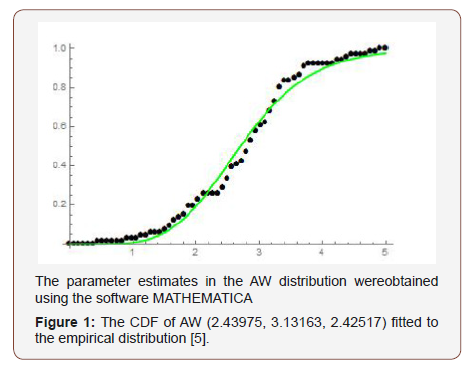
Illustration of A_T − X (W) Family of Distributions of type I

The data set refers to the remission times (in months) of a random sample of 128 bladder cancer patients studied in [6]. We assume the random variable T follows the Burr X (BX) family of distributions so that for t, a, b > 0, the CDF is given by

and the PDF is given by

We assume the random variable X is Lomax distributed so the for x, c, d > 0, the CDF is given by

and the PDF is given by

Now we consider Remark 4.3 in Definition 4.2, then we get the following

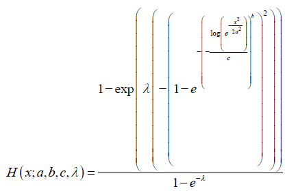
Theorem 5.3: The CDF of the A_BurrX−Lomax family of distributions, for x,a,b,c,d,λ > 0 is given by

Remark 5.4: If a random variable W has CDF given by the ABurrX − Lomax family of distributions, we write W  ABXL(a,b,c, d,λ ) (Figure 2).

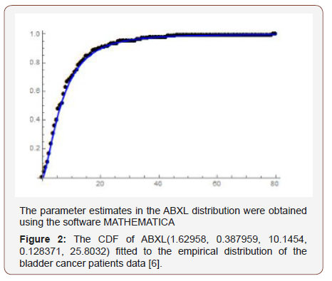
Illustration of A_T − X (W) Family of Distributions of type II

The second data set is on 30 successive March precipitation (in inches) observations obtained from [7] and recorded in Section 7 of [8]. We assume the random variable T with support [0,∞) follows the Weibull distribution, so that for t > 0, and b, c > 0, the CDF is given by

and the PDF is given by

We also assume the random variable X follows the Rayleigh distribution, so that for x, a > 0, the PDF is given by

and the CDF is given by

Considering Remark 4.5 in the first integral of Definition 4.4, we get the following Theorem 5.5. The CDF of the AWeibull − Rayleigh family of distributions of type II is given by

Remark 5.6: When a random variable J* has CDF given by Theorem 3.5, we write J* ~ AWR(a,b,c,λ) (Figure 3).

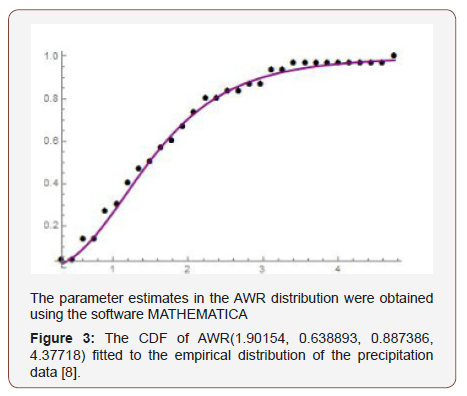
Illustration of A_T − X (W) Family of Distributions of type III

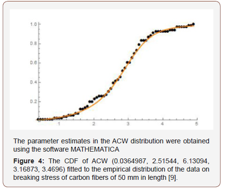
In this application we consider the data set in [9] from [10], on the breaking stress of carbon fibers of 50 mm in length. We assume the random variable T with support (−∞,∞) follows the Cauchy distribution, so that for t, a 2 R, b > 0, the CDF is given by

and the PDF is given by

We also assume the random variable X follows the Weibull distribution, so that for x > 0, and c, d > 0, the CDF is given by

and the PDF is given by now considering Remark 4.7 in the second integral of Definition 4.6, we get the following

Theorem 5.7: The CDF of the ACauchy − Weibull family of distributions of type III is given by

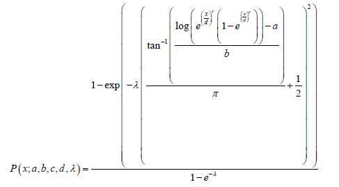
Where x;a,b,c,d,λ > 0

Remark 5.8: By differentiating the CDF of the A_Cauchy−Weibull family of distributions of type III, the PDF can be obtained

Remark 5.9: When a random variable N* has CDF given by Theorem 5.7, we write (Figure 4) N* ~ ACW (a,b,c,d,λ)

None.

No conflict of interest.

1. Ayman Alzaatreh, Carl Lee, Felix Famoye (2013) A new method for generating families of continuous distributions. METRON 71: 63-79.
2. Ahmad Z (2018) The Zubair-G Family of Distributions: Properties and Applications. Ann Data Sci: 1-14.
3. Ristic MM, Nadarajah S (2014) A new lifetime distribution. J Stat Comput Simul 84: 135-150.
4. Mahmoudi E, Sepahdar A (2013) Exponentiated Weibull-Poisson distribution: Model, properties and applications. Math Comput Simul 92: 76-97.
5. Ayman Alzaatreh, Carl Lee, Felix Famoye (2014) T-normal family of distributions: a new approach to generalize the normal distribution. Journal of Statistical Distributions and Applications 1: 16.
6. Lee ET, Wang JW (2003) Statistical Methods for Survival Data Analysis (3rd ed.), Wiley, New York, USA.
7. Hinkley D (1977) On quick choice of power transformation. Applied Statistics 26(1): 67-69.
8. Muhammad Ahsan ul Haq (2016) Transmuted Exponentiated Inverse Rayleigh Distribution. J Stat Appl Pro 5(2): 337-343.
9. Maalee Almheidat, Felix Famoye, Carl Lee (2015) Some Generalized Families of Weibull Distribution: Properties and Applications. International Journal of Statistics and Probability 4(3).Nicholas MD, Padgett WJ (2006) A bootstrap control for Weibull percentile. Quality and Reliability Engineering International 22(2): 141- 151.
10. Nicholas MD, Padgett WJ (2006) A bootstrap control for Weibull percentile. Quality and Reliability Engineering International 22(2): 141- 151.