Analysis of Growth Performance Data in Sidama Goats using Fixed and Random Regression Models

Based upon the species of farm animals, several traits such as milk yield, body weight gain, feed intake and longevity are used for selection of candidate animals as the genetic evaluation is practiced [1]. As mentioned by Meyer [2] growth of animals is a prime example of a trait measured repeatedly per individual along a continuous scale (time) which changes gradually and continually and can be modelled using random regressions [3]. In any meat producing goat industry, body weight and average daily gain are considered to be important components for market meat production. Random regression models have been utilized to describe a linear mixed model including appropriate covariates to model the effect of time on repeated records as fixed and random terms [4]. Using random regression models there is no need to correct towards certain landmark ages [3].

The objectives of this study were to compare the growth curve of animals in different treatments and to evaluate the differences in body weight gains caused by the different rations in the treatments and their implications on choosing a ration.

Description of the study area

This study was conducted at Dilla Agricultural, Technical, Vocational, Education and Training College, which is situated 365 km south of Addis Ababa, Ethiopia. The area lies at a latitude of 6° 27’ N and 38° 30’ E longitude with an altitude ranging from 1550- 1700 m.a.s.l. The mean annual temperature is 20.7° C and relative humidity ranging from 60-70%. The annual rainfall varies between 1100-1300mm.

Experimental animals and treatments

In this experiment a total of 25 male intact Sidama goats with a live weight of 15.13kg ± 1.4 (mean ± SD) were purchased from the local market and stayed in quarantine house for three weeks. The goats were treated against internal and external parasites. They were housed in individual pens with access to individual feeding and watering troughs.

Experimental feeds and treatments

Grass hay (having a crude protein [CP] of 9.2%) and leaves from Erythrina brucei trees (CP ≈ 25.7%) were made available for this experiment from the study area. Cotton seed meal (CP ≈ 45.3%) was purchased from nearby oil processing plant.

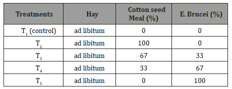
The experimental animals were divided into five animals per treatment. The treatments consisted of hay (control, T1) and hay supplemented with 300 g DM/day/head of cotton seed meal and E. brucei leaf combined in different proportion (Table 1).

Table 1: Experimental treatments and proportions of feeds used.

Body weight measurements

Following a three week acclimatization period, growth data were collected over an 80-day feeding trial. Each goat was weighed at the beginning of the experiment (initial body weight, IBW) and every successive ten-day thereafter. All goats were weighed during morning hours after overnight fasting using suspended weighing scale having sensitivity of 100 grams.

Model selection approaches

Growth traits such as body weight and average daily gains are important response indicators in goats. The typical repeated measures experiment in animal research consists of animals randomly assigned to different treatments and with responses measured on each animal over a sequence of time points. In this study, for the analysis of growth traits, repeated records of body weight gain were collected.

Responses measured on the same animal over a sequence of time points are correlated because they contain a common contribution from the animal. Moreover, measures on the same animal close in time tend to be highly correlated than measures far apart in time. Also, variances of repeated measures often change and increase steadily with time. Since the potential patterns of correlation and variation may combine to produce a complicated covariance structure, these feature of repeated measures data require special methods of statistical analysis [5]. Standard regression and ANOVA methods may produce invalid results because they require mathematical assumptions that do not hold with repeated measures data.

The general linear mixed model allows the capability to address these issues directly by using the MIXED MODEL procedure of the SAS System [6]. Thus, in this study, for analyzing the data on repeated records of body weight gains using linear mixed model a two-step modelling approach was used. The first step models and compares the expected value structure by using the ML Method, while the second step models and compares the covariance structure by using the REML Method [6,7].

Modelling the expected value structure

Depending on the age of animals, the description of growth traits like body weight and average daily gains can be modelled using polynomials of 1_st-5_th degree [8-10].

In this first step, the selection of an optimum model for the expected value structure is found by incorporating fixed effects to be tested in the different models through the use of fixed regression model where selection of an optimum model is carried out by considering uncorrelated residual effects and homogenous variance assumptions.

In order to realize this, we make use of the modelling approach applied by polynomials. This approach requires n covariates. Let t_max be the maximal length of feeding period (in this study, t_max = 80 days). In an attempt to achieve better convergence properties, the covariates are expressed as a function of the standardized dayson- test, i.e., t = DT/t_max (with DT = days-on-test). It holds true that: x₀(t) = 1.0, x₁(t) = t; x₂(t) = t²; and x_n(t) = tⁿ. These covariates are well-suited for the description of growth curves. Furthermore, it is possible to stay within the class of linear models.

Accordingly, the body weight gain of goat l, from treatment i, having an initial body weight of j, on days-on-test of k for the standardized days-on-test t = t_ijkl/t_max is given by:

In this working model, bi0 to bin stand for fixed regression coefficients of treatment i, x(t) = (1, t, t ² , t³, t ⁿ ) is the vector of covariates formed according to polynomials and represents random residual effects.

By the comparison and finally selection of an optimum model using the above polynomial models, the aim will be to find the best order of fit for the fixed regression on age to model population trajectory.

In contrast to the usual modelling of experimental effects, the effect of treatment in {1} is modelled by the respective fixed regression coefficients. Thus, differences between the treatments are expressed by different patterns of the growth curves. The resulting flexibility can be used for the calculation of average body weight gains for different sub-periods of the growth time. For the analysis of the data with model {1}, the following SAS statement can be used:

PROC MIXED DATA=GOAT METHOD=ML;

CLASS TRT DT;

MODEL BWG = TRT IBW DT X₁(TRT) X₂(TRT) ... X_n (TRT)/ NOINT;

In the MODEL-statement X₁, …, X_n are the covariates for the description of the different treatment specific growth curves. By using the option NOINT, the general mean is estimated together with the treatment effects.

Modelling the covariance structure

In this second step, the selection of an optimum model for the covariance structure is done by using the optimum model chosen for the expected value structure (sections “Modelling the Expected Value Structure”) and then by incorporating the random effect part (i.e. additive genetic effect of an animal) in the different models to be tested. This is realized by using random regression model (RRM) where selection of an optimum model for the covariance structure is accomplished by considering correlated residual effects and heterogeneous variance assumptions. The classical random regression model involves a random intercept and slope for each subject.

Dependencies between repeated body weight gains of a goat have to be modelled with the help of covariance structures. In order to realize this, goat specific random regression coefficients al0 – aln are introduced as deviations from the fixed regression coefficients, where the value of n should not be greater than that found for the optimum model of the expected value structure.

Let al = (a_l0, …, a_ln)’ be the vector of the random regression coefficients of goat l and let x = (x₀, x₁, …, x_n)’ be the vector of the covariates. Then, the following random regression model for dayson- test can be written from {1}:

In model {2}, all random effects are assumed to be normally distributed with a mean value of 0. Additionally, we assume that all random effects associated with different goats are generally independent of each other. By using the covariate matrix Al and the residual variance between body weight gains of a goat at time point t₁ and t₂

Furthermore, all goats in model {2} were treated as unrelated. For the vectors of the random regression coefficients of two goats l and l*, it follows: cov(a_l, a´_l*) = 0. The following SAS statements can be used to analyze the data with model {2}:

PROC MIXED DATA=GOAT METHOD=REML;

CLASS TRT DT GOAT;

MODEL BWG = TRT IBW DT X₁(TRT) X₂(TRT) ... X_n(TRT)/ NOINT;

RANDOM INT X₁ X₂ ... X_n/SUBJECT=GOAT TYPE=UN;

If n=0 in model {2}, this means that one random effect per goat is included and that the covariance function in {3} is of the form:

Here, δ₁₂ =1 for t₁ = t₂ ; in all other cases, δ₁₂ = 0 . Because of the above formula, all pairs of measurements on the same goat have the same correlation. Thus, the correlation between two measures at time t₁ and t₂ is:

Up to now, the covariance structure has been modelled by using goat specific random effects only. In the following, the residual covariance structure of model {2} will be extended further [2].

Let e(t) be the residual effect of a goat for the body weight gain on days-on-test of t. Then, let us use the following model: e(t) = e₁(t) + e₂(t). Here, e₁(t) stands for the component of the serial correlation between repeated measurements for a goat, e2(t) denotes the component for the residual error with equal variance for all measurements. The residual effects for the latter are assumed to be independent and identically distributed. The model for the serial covariance structure is completed by adding a distance correlation function g. This function is selected in such a way that all residual effects e1(t) of a goat have the same variance and that the correlation between two such effects is always positive but decreases monotonically with increasing temporal distance between two measurements for the same goat. Then, the variance and covariance function of the residual effects of a goat are given by:

Here, is the temporal distance between two measurement points. Frequently used functions are the Gaussian function and the exponential serial correlation function:

The two functions are always positive and decrease monotonically with increasing temporal difference d. They are continuous at d = 0 and meet the requirement that g(0) = 1. In {5}, ρ is an unknown parameter greater than 0. The smaller the value of ρ, the stronger the function g decreases with increasing value of d. Model {2}, extended with the exponential correlation function, can be fitted with the following SAS statements:

PROC MIXED DATA=GOAT METHOD=REML;

CLASS TRT DT GOAT;

MODEL BWG = TRT IBW DT X1(TRT) X2(TRT) ... Xn(TRT)/NOINT;

RANDOM INT X₁ X₂ ... X_n/SUBJECT=GOAT TYPE=UN;

REPEATED/SUBJECT=GOAT TYPE=SP(EXP)(TIME) LOCAL;

Once the optimum model for the covariance structure is found in this second step, then the analysis of time trends for treatments by estimating and comparing means (i.e., tests of fixed effects) can be done with the help of t- and F-tests (Tukey-Tests) [5,11,12].

With regard to practical applications, the choice of statistical models is of greatest importance. In the next sections, the use of Likelihood-Ratio Tests and information criteria for model selection will be illustrated.

Likelihood-ratio test (LRT)

The LRT is a statistical test of the quality of fit of two hierarchically nested models. A model is hierarchically subordinated to another model if the former can be reduced to a special case of the latter by setting one or more of its parameters to zero or to fixed values. Therefore, the subordinated model is denoted as restricted and the hierarchically higher model is denoted as unrestricted. The null hypothesis is that both models are the same (extra parameters do not improve the fit). If we fail to reject the null hypothesis, the restricted model, because of its simpler form (and yet, its comparable explanatory power), is to be preferred. The likelihood ratio test is used to make sure that the unrestricted model indeed returns a (significantly) better result than the restricted model.

The likelihood ratio test statistic is given by:

The LRT statistic approximately follows a chi-square distribution. The degrees of freedom are equal to the number of restrictions in the extended model, which means that model (s) can be obtained as a special case of (g). Thus, the degrees of freedom are given by the number of variance components that need to be set to zero in the general model (g) to obtain the restricted model (s).

There has been concern that the use of LRT to determine the “best” model to fit the data might favor over parameterized models, thus this test does not favor parsimonious models. This led to the use of information criteria – sometimes also referred to as penalized likelihoods - which adjust for number of parameters estimated and sample size.

Information criteria

For the comparison of models without hierarchical structures, the information criteria of Akaike [13-15] and its modification by Hurvich & Tsai [16,17] and also the criterion by Schwarz [18-21] can be used.

When using the Maximum-Likelihood (ML) method, the calculations of these criteria for comparing the expected value structure are given by:

Here, pX is the rank of the design matrix X for the fixed effects, q is the number of variance components to be estimated and n is the number of records per animal.

The comparison of the covariance structure by identical expected value structure will be done using the Restricted Maximum-Likelihood (REML) method and the calculations of the criteria are given by:

Both criteria (i.e., AICC and BIC) use the number of variance components as penalty to balance the log-likelihood value. The penalty imposed by BIC is more severe than that imposed by AICC. The best model (of all competing models) is the one with the lowest criterion value. The ranking of models by their AICC or BIC values assumes the existence of identical fixed parameter structures in all competing models [22,23].

A comparison of the criteria shows, AICC tends to prefer complex models while that of BIC tends to prefer simpler models for selection.

Descriptive statistics

A summary results of the data on body weight gain over the different sub-periods, i.e. from day 10 (t₁₀) up to day 80 (t₈₀), is given in the table below.

Table 2: Descriptive statistic results of body weight gain (kg) of goats across the five treatments measured on eight consecutive times (t₁₀ to t₈₀).

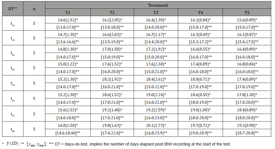
The results shown in Table 2 reveal differences in body weight gain among the different treatments. This was expected as the proportions of feed ingredients differed across treatments resulting in different nutritional compositions.

With repeated measures data, an obvious first graph to consider is the scatter plot of the weight of animals against time. Means plotted in Figure 1 show increase in body weight gains over time for all treatments slowly and steadily with age. One can see a clear difference of the body weight gain records at different measurement times.

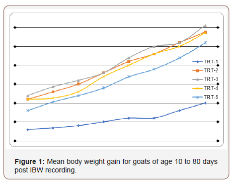
The profile for treatment T1 (the basal diet) shows body weight gains less than for other treatments (i.e., treatments T2, T3, T4 and T5) on all days. Profiles for treatments T2, T3, T4 and T5 show considerable increase in body weight gain corresponding to increases in dietary supplement feeding.

Modelling the expected value structure

The table below gives the results found for the different models tested to find an optimum model for the expected value structure. The summarized models given in the table are analysis results from the fixed regression model with uncorrelated residual effects and homogenous variance assumptions.

It is to emphasize that decisions made here only apply in relation to the expected value structure but not on the confidence interval and significance tests of the fixed effects used in the model. That is possible only after optimization of the covariance structure has been done.

As can be seen from the results in the above table, four models, i.e. M1, …, M4, are given in increasing order of complexity. In this regards M1 is only given as a demonstration purpose to show the development of the different models tested. This model does not allow a time-dependent estimation of the model effects.

According to the -2logL, AICC and BIC values given for the four models, M1 is found to be the least chosen, as it has the largest values for -2logL, AICC and BIC. A substantial decrease in the values of -2logL, AICC and BIC can be seen for the other models (M2, M3, and M4), where the decrease in M4 is the highest so that this model is chosen to be the optimum model. The models M1, …, M3 can be seen as special cases of M4 that are found through substituting one or more fixed effects in M4 by zero.

Testing of additional models beyond M4 with a quadratic and above polynomial for the effect of treatment has led to no improvement in decreasing the values of AICC and BIC as was the case in M4. As a consequence, considering quadratic and above polynomials is left out.

Modelling the covariance structure

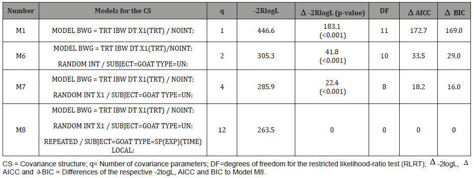
The table below gives the results found for the different models tested to find an optimum model for the covariance structure. The summarized models (M5, …, M8) given in the table below are analysis results from the random regression model with correlated residual effects and heterogeneous variance assumptions.

As can be seen from the results in the above table, four models, i.e. M5, …, M8, are given in increasing order of complexity. According to the -2logL, AICC and BIC values given for these models, M5 is found to be the least chosen, as it has the largest values for -2logL, AICC and BIC. A substantial decrease in the values of -2logL, AICC and BIC can be seen for the other models (M6, M7, and M8), where the decrease in M8 is the highest so that this model is chosen to be the optimum model. The models M5, …, M7 can be seen as special cases of M8 that are found through substituting one or more random effects in M8 by zero. Besides, the analysis results of the restricted likelihood ratio test show a significant improvement as one goes from M5 to M8 even though the number of model parameters increased from 1 in M5 to 12 in M8.

Comparing table 3 vs. 4, a considerable decrease in the values of the estimates for -2logL, AICC, and BIC has been achieved in table 4 (RRM) than table 3 (FRM). Hence random regression models fit the data better than fixed regression models. Random regression models took into account that measurements are not all done at the same age.

Table 3: Estimated error variance (σˆ² _e ), with -2 multiplied Log-Likelihood function (-2logL), results of LRT and differences for the information criteria AICC and BIC.

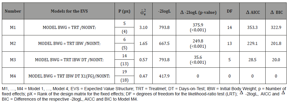
Table 4: With -2 multiplied restricted Log-Likelihood (-2RlogL), Results of LRT and differences of the information criteria AICC and BIC.

Once the covariance structure has been chosen the results for the tests of fixed effects can be interpreted.

Tests of fixed effects: Comparing the effect of treatments on body weight gains

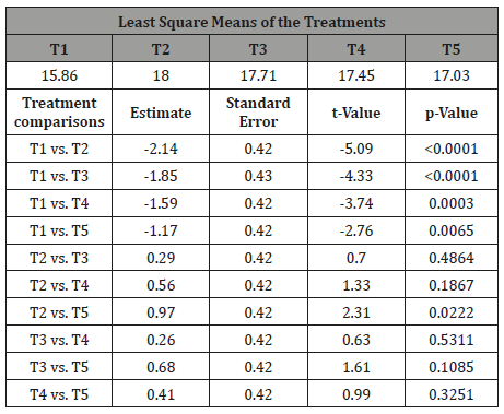
T1 compared with other treatments (i.e. T2, T3, T4 and T5) has a significantly lower body weight gain. This supports the fact that raising the level of crude protein in treatments T2, …, T5 has resulted a significant increase of body weight gain.

There was no significant difference in body weight gain between T2 and T3. Similarly, no significant difference in body weight gain was observed between T2 and T4. Since the proportion of cottonseed- meal and E. brucei across these treatments is different (i.e. T2 > T3 > T4), the cost of the rations for these treatments also differ (i.e. cost of the ration for T4 < T3 < T2). Thus, from least cost feed formulation point of view T4 is better to recommend than T2 and T3.

T4 vs. T5 has no significant difference in body weight gain. However, since T4 has some proportions of cotton-seed-meal in the ration, the cost of T4 is more than that of T5. Thus, again from least cost feed formulation point of view T5 is better to recommend than T4.

This work demonstrated the nutritive potential of E brucei leaves relative to cotton-seed-meal through conventional feeding trials. The conclusions made above need to be confirmed on further studies. Further studies on Sidama goats and other related breeds are necessary to provide sufficient information as to the decision to be made regarding the choice of an optimum level of E. brucei in relation to achieved body weight gain and cost of the ration (Table 5).

Table 5: Comparison of the effect of treatment on body weight gain.

None.

No conflict of interest.

1. Akbas Y, C Takma, E Yaylak (2004) Genetic parameters for quail body weights using a random regression model. South Af J Anim. Sci 34(2): 104-109.
2. Meyer K (1999) Random regression models to describe phenotypic variation in weights of beef cows when age and season effects are confounded. Proceedings of the 50th Annual Meeting of the European Association for Animal Production, Zurich, Switzerland, 22-26, Session G3.2.
3. Meyer K (2004) Scope for a random regression model in genetic evaluation of beef cattle for growth. Live Prod Sci 86(1-3): 69-83.
4. Schaeffer LR, JCM Dekkers (1994) Random regressions in animal models for test-day production in dairy cattle. In: Proceedings of the 5th World Congress on Genetics Applied to Livestock Production, Guelph, Ontario, Canada 18: 443-446.
5. Little RC, Henry PR, Ammerman CB (1998) Statistical analysis of repeated measures data using SAS procedures. J Animal Sci 76(4): 1216- 1231.
6. SAS Institute Inc (2005) SAS/ STAT Software Release, User’s Guide, Version 9.1.3.
7. Ngo L, Brand R (1997) Model Selection in Linear Mixed Effects Models Using SAS Proc Mixed. SAS Users Group International (22) San Diego, California March 16-19.
8. Albuquerque LG, Meyer K (2001) Estimates of covariance functions for growth from birth to 630 days of age in Nelore cattle. J Anim Sci 79(11): 2776-2789.
9. Meyer K (2001) Estimates of direct and maternal covariance function for growth of Australian beef calves from birth to weaning. Genet Sel Evol 33(5): 487-514.
10. Nobre PRC, Misztal I, Tsuruta S, Bertrand JK, Silva LOC, et al. (2003a) Analysis of growth curves of Nelore cattle by multi-trait and random regression model. J Anim Sci 81(4): 918-926.
11. Fai AHT, Cornelius PL (1996) Approximate F-Tests of multiple degree of freedom hypotheses in generalized least squares analyses of unbalanced split-plot experiments. Journal of Statistical Computation and Simulation 54: 363-378.
12. Giesbrecht FG, Burns JC (1985) Two-stage analysis based on a mixed model: large-sample asymptotic theory and small-sample simulation results: Biometrics 41(2): 477-486.
13. Akaike H (1969) Fitting autoregressive models for prediction. Annals of the Institute of Statistical Mathematics 1(21): 243-247.
14. Akaike H (1973) Information theory and an extension of the maximum likelihood principle. 2nd International Symposium. Information theory. Petrov BN, Csaki F (eds) Akademiai Kiado, Budapest, Hungary pp. 267- 281.
15. Akaike H (1974) A new look at the statistical model identification. IEEE Transactions on Automatic Control 19(6): 716-723.
16. Hurvich CM, Tsai CL (1989) Regression and time series model selection in small samples. Biometrika 76(2): 297-397.
17. Wolfinger RD (1993) Covariance structure selection in general mixed models. Communications in Statistics - Simulation and Computations 22(4): 1079-1106.
18. Arango JA, LD Van Vleck (2002) Size of beef cows: Early ideas, new developments. Genet Mol Res 1(1): 51-63.
19. Kenward MG, Roger JH (1997) Small sample inference for fixed effects from restricted maximum likelihood. Biometrics 53(3): 983-997.
20. Lesaffre E, Todem D, Verbeke G, Kenward M (2000) Flexible modelling of the covariate matrix in a linear random effects model. Biometr J 42(7):807-822.
21. Schwarz G (1978) Estimating the dimension of a model. Annals of Statistics 6(2): 461-464.
22. Spilke J, Piepho HP, Hu X (2005) A simulation study on tests of hypotheses and confidence intervals for fixed effects in mixed models for blocked experiments with missing data. Journal of Agricultural, Biological and Environmental Statistics 10(3): 374-389.
23. Verbeke G, Lesaffre E, Brandt LJ (1998) The detection of residual serial correlation in linear mixed models. Statistics in Medicine 17(12): 1391- 1402.