Kinematic Modeling and Simulation of Inverted Pendulum for Balancing a Two-Wheeled Robot

Benefits of two-wheeled robots

Several two wheeled robots have been designed and a variety of control methods have been proven successful at stabilizing and controlling a two wheeled pendulum base. These methods include Sliding Mode [1,2], PID [3], Linear Quadratic Gaussian [4,3], and Evolutionary Fuzzy Control through “an adaptive fusion of continuous ant colony optimization and particle swarm optimization” [5]. While all the control systems have been tested using software simulation, most have not been subjected to real world evaluation.

However, those that have been tested in the real world have demonstrated several unique capabilities and functional areas where the two wheeled mobile robot design excels: dynamic stabilization and maneuverability.

Dynamic stabilization increases a robot’s ability to handle large shifts in the center of gravity [4]. This has been demonstrat ed to lead to robots that are better at handling heavy objects with a smaller support base than a robot dependent on static stability, such as a stationary arm or a three or more wheeled robot [6]. This alsoimproves impulse response during navigation and allows for end-effectors attached to two-wheeled robots to have a wider range of motion than end-effectors attached to four-wheeled robots of the same size. Maneuverability results from the narrower ground footprint and allows for greater performance on uneven surfaces in confined spaces [3] when compared to four-wheeled robots. Combined with dynamic stabilization, a two-wheeled robot is a robust mobile design that has the potential to be more versatile than a four-wheeled robot in most situations.

Mathematical model of two wheeled robot

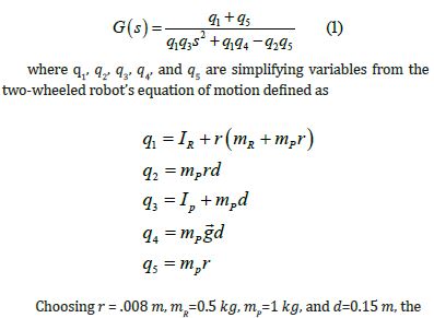
As discussed in [7], a robot’s physical parameters, such as the wheel diameter, the mass of the platform and wheels, and the distance between the center of rotation and the center of gravity, have a strong influence on the robot’s controllability. Therefore, the development of a two wheeled robot must begin with the mathematical model for a generic two wheeled robot. Such a model will allow combinations of parameters to be tested to inform the physical design of the robot. This will also allow the effect of a controller to be tested on various physical configurations and ideal physical ratios to be extracted.

The two major components of motion for a two-wheeled robot are navigation and balance. The mathematical model required for navigation is the kinematic model of a two wheeled robot. The mathematical model for balance is an inverted pendulum as found in [7]. This paper will focus on developing a controller to stabilize the robot’s balance.

1. Nomenclature

A. Variables

• 𝐶 Center

• 𝑑 Vertical distance from the point of rotation to the platform’s center of gravity (m)

• 𝐷(𝑠) System controller in 𝑠 domain

• 𝑒𝑠𝑠 Steady state error

• 𝑔⃗ Gravity (𝑚𝑠2)

• 𝐺(𝑠) System plant in 𝑠 domain

• 𝐼 Moment of inertia (𝑘𝑔 𝑚2)

• 𝑗 √−1, Imaginary number

• 𝐾 Proportional gain

• 𝐾𝑝 Proportional error constant in step response steady state error

• 𝑚 Mass (𝑘𝑔)

• 𝑝 Pole of a transfer function, root of the characteristic equation

• 𝑃𝑂 Percent overshoot (%)

• 𝑞 Simplifying variable

• 𝑞(𝑠) Characteristic equation, which is the denominator of a transfer function

• 𝑟 Radius of the wheel (𝑚)

• 𝑅(𝑠) System input in s domain

• 𝑠 Complex frequency, 𝑗 𝜔, generally associated with the Laplace transformation

• 𝑇𝑠 Settling time (to within 2% of the final value)

• 𝑋 x-axis (parallel to the ground, forms a horizontal plane with the y-axis)

• 𝑌(𝑠) System output in s domain

• 𝑧 Zero of a transfer function, the root of the function’s numerator

• 𝑍 z-axis (vertical axis, defined as perpendicular to the ground and increasing upward)

B. Subscripts

• 1,2,… 1st, 2nd, etc. of the attached variable

• 𝑔⃗ Gravity (𝑚𝑠2)

• 𝑃 Platform reference frame

• 𝑅 Robot base’s reference frame

• 𝑠𝑡𝑒𝑝 Step Input

C. Greek Variables

• 𝜖 A very small number greater than zero which replaces a 0 in the first column of a Routh Array.

• 𝜂 Angle from vertical (angle between the robot’s z-axis and the platform’s z-axis)

• 𝜏 Torque

• 𝜁 Damping ratio of the system

• 𝜔𝑛 Natural frequency of the system (Hz)

(Figure 1) The controller and two-wheeled robot system was defined as shown in Figure 1, with the plant, 𝐺(𝑠), describing the relationship between the motor torque and the system angle from vertical (𝜂 in Figure 2), the controller, 𝐷(𝑠), to be developed in this research, and the feedback, 𝐻(𝑠)=1, to be integrated in future work. The plant transfer function was developed using the small angle approximation for linearization with zero initial conditions during the Laplace transformation [7] (Figure 2).

Plant transfer function

As shown in [7], the plant, defined by an analysis of the system starting from first principles, is

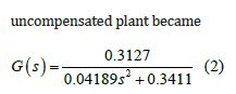
which had roots at 𝑠=0 ± 𝑗2.85, as shown in the Root Locus of the uncompensated system (Figure 3), and the system response to step input shown in Figure 4 (Figure 3).

Uncompensated system stability

As defined in [8], the Routh-Hurwitz Criteria states that there will be sign changes in the first column of the Routh array if a system’s characteristic equation has roots with positive real parts and that the number of such roots will equal the number of sign changes in the first column of the array. The characteristic equation for the uncompensated system is 𝑞(𝑠)= 1+𝐷(𝑠)𝐺(𝑠), where 𝐷(𝑠)=𝐾 and 𝐺(𝑠) is the plant transfer function defined in Error! Reference source not found. [8]. Therefore, the characteristic equation of the uncompensated system is 𝑞(𝑠)=0.04189𝑠²+0.3411+0.3127𝐾, which has the Routh array:

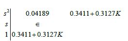
The 𝜖 is necessary to replace the 0 resulting from the lack of a first order term in the characteristic equation. The array demonstrates that the system is only marginally stable for any 𝜖>0 and 𝐾>−0.3411/0.3127=−1.09.

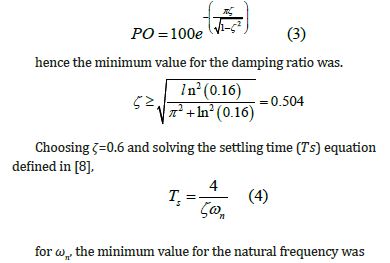
The system response to step input was examined since this most closely resembles the input likely to be experienced by the system. The desired system response should exhibit no more than 16% overshoot (𝑃𝑂_{𝑠𝑡𝑒𝑝}≤16%), have a settling time of no more than 2 seconds to reach 2% of the final value (𝑇_{𝑠,𝑠𝑡𝑒𝑝}≤2𝑠), and the final value should be no more than 5% from the desired final value (_{𝑒𝑠𝑠,𝑠𝑡𝑒𝑝}≤0.05).

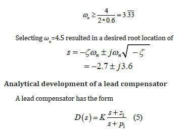
Desired root location

The uncompensated system requires shifting to the left to achieve stability, so a lead compensator was developed. The minimum values of the system damping ratio and natural frequency were calculated from the design specifications. In [8], percent overshoot is defined as

Analytical development of a lead compensator

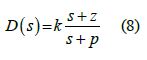
A lead compensator has the form

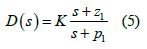
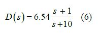
Usually, 𝑧₁ is chosen to be coinsident with a plant pole to cancel the pole, which will shift the root locus left. Then 𝑝1 is either chosen to create a more stable system or defined using the phase angle criterion if the plant has multiple poles. However, since the plant has complex roots, a value for 𝑧₁ cannot be chosen to cancel out existing poles in the plant. Therefore, 𝑧₁=1 and 𝑝1=10 were selected through trial and error, which meant that 𝐾= 6.54, using magnitude criterion, and the controller had the form

A Matlab script was used for iteration and the best step response that could be achieved utilizing only a lead compensator is shown in Figure 5.

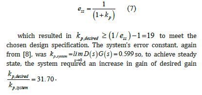
Steady state analysis

To meet the steady state requirement the desired error constant (𝑘𝑝) was defined by considering the steady state error equation from [8]

D. Analytical Development of Lag Compensator

To apply the gain a lag compensator was developed. A lag compensator has the form

where |𝑧|/|𝑝| <1, |𝑠+𝑧|=𝑝, and the error constant, 𝑘𝑝, increases by a ratio of 𝑧/𝑝,. Keeping the previously determined gain, the lag compensator zero is defined [8] as 𝑧=𝛼/10 where 𝛼 is the centroid of the uncompensated system. For the lead compensated plant 𝛼=−9 (𝛼=0 for the uncompensated plant), so 𝑧 =−0.9. The pole is defined as being significantly less than the ratio of the zero to the desired gain, so

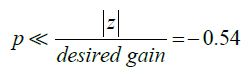
Choosing 𝑝=0.02 results in the lag compensator.

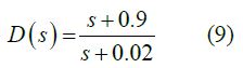
which, when applied to the lead compensated system, resulted in the step response shown in Figure 6 and the Root Locus shown in Figure 7 (Figure 6).

Simulation development of lead-lag compensator

Matlab’s built in Control System Designer Optimization function was also used to generate a controller. Starting with the analytically derived gain, poles, and zeros as initial values, the optimization function was set to optimize each to achieve a settling time of less than 2 seconds and no more than 16% overshoot. The resulting lead-lag compensator was

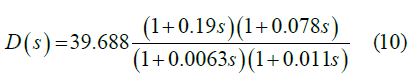
which had the step response shown in Figure 10. The fully compensated system had the Root Locus shown in Figure 8 and the Bode Plots shown in Figure 9 (Figure 8,9 & 10).

Subjecting the system to step input illustrates the system response to external stimuli, such as gravity in the two-wheeled robot’s case. The analytically developed lead-lag compensator resulted in a percent overshoot of 𝑃𝑂𝑠𝑡𝑒𝑝=32% and a settling time of 𝑇𝑠=2.89𝑠 which did not meet the transient design requirements. The lead-lag compensator developed using Matlab’s Control System Designer did meet the desired design parameters with a percent overshoot of 𝑃𝑂𝑠𝑡𝑒𝑝=9.96%, a settling time of 𝑇𝑠=0.43𝑠, and a steady state error of 𝑒𝑠𝑠,𝑠𝑡𝑒𝑝=0.03 in response to step input. Comparing the analytically developed lead-lag compensator to the one developed using Matlab’s Control System Designer illustrates the challenges involved in analytically developing system controllers as well as the importance of understanding controller development methods. Due to the nonlinear nature of the plant equation more advanced controller development methods, such as sliding mode control as discussed in [1] [2], are more commonly applied to balancing a two wheeled robot than lead-lag compensators.

Future work should focus on implementing disturbance rejection to compensate for unexpected bumps or inputs as well as integrating a sensor feedback mechanism to develop a more robust controller. It should be incorporated with a navigation system to provide balance during transit as well as while the robot is stationary. Finally, it should also include experimental testing of the simulation developed controller on a physical system to fully evaluate its ability to stabilize a two-wheeled robot.

None.

None.

1. Y Zhou, Z Wang (2016) Robust motion control of a two-wheeled inverted pendulum with an input delay based on optimal integral sliding mode manifold. Nonlinear Dynamics 85(3): 2065-2074.
2. N Esmaeili, A Alfi, H Khosravi (2017) Balancing and Trajectory Tracking of Two-Wheeled Mobile Robot Using Backstepping Sliding Mode Control: Design and Experiments. Journal of Intelligent & Robotic Systems; Dordrecht 87(3-4): 601-613.
3. Onkol, C Kasnakoglu (2015) Modeling and Control of a Robot Arm on a Two Wheeled Moving Platform. Applied Mechanics and Materials 789-790: 735-741.
4. C Kasnakoğlu, M Önkol (2018) Adaptive Model Predictive Control of a Two-wheeled Robot Manipulator with Varying Mass," Measurement and Control 51(1-2): 38-56.
5. CF Juang, MG Lai, WT Zeng (2015) Evolutionary Fuzzy Control and Navigation for Two Wheeled Robots Cooperatively Carrying an Object in Unknown Environments. IEEE Transactions on Cybernetics 45(9): 1731-1743.
6. M Stillman, J Olson, W Gloss (2010) Golem Krang: Dynamically stable humanoid robot for mobile manipulation," in IEEE International Conference on Robotics and Automation (ICRA), Anchorage, AK, USA.
7. K Remell (2021) Mathematical Modeling of a Two Wheeled Robotic Base (Mechanical Engineering Undergraduate Honors Theses)," 26 May 2021. [Online]. Available: https://scholarworks.uark.edu/meeguht/96/. [Accessed 8 July 2020].
8. R C Dorf, R H Bishop (2011) Modern Control Systms, 12 ed., Upper Saddle River, New Jersey: Pearson Education.
9. MM Rahman, Ashik-E-Rasul, H Nowab Md Aminul, M Hassan, I M Hasib, et al. (2011) Development of a two wheeled self balancing robot with speech recognition and navigation algorithm in International Conference on Mechanical Engineering, BUET, Dhaka, 2016.