Understanding The Structure and Parameters Identification of Compliant Robot Arms Using Frequency Domain Analysis

The robot arms based on rotary electric brushless motors are widely used for various robot configurations – horizontal (SCARA) or vertical (PUMA) configurations. This is thanks to its high dynamics owing low moments of inertia and high energy efficiency compared to any other type of electric motors. The dynamic performance of the robot axes is different from ones of other servo systems namely in the lower range of first resonance (Figure 1). Further its improvement is limited by the mechanical resonance. Proper control design of such axes is based on an identification procedure from choosing a model of an electromechanical structure with further parameters identification. We must point out that choosing a model is one of the more important and complex tasks of robots’ arms design.

The existence of resonances due to compliant linkages is represented by pick-ups and pick-downs for each resonance (Figure1). It is considered that pick-downs are Anti-Resonance (AR), and pick-up frequencies are Resonance (R) frequencies.

The pairs of AR and R frequencies represent a well-known compliant reducer type of resonance [1]. The Bode plots of a compliant reducer have key features [2] namely
• AR frequency is lower than R frequency.
• Bode phase increasing up to (+180°) between AR and R frequencies.
• AR frequencies are ones with “rigid” attachment of motor.
• Mismatch ratio (ratio of bodies’ moment of inertia) of each resonance is defined by the second power of R to AR frequency ratios.
• the Bode amplitudes increases after each resonance where amplitude increment L is defined by the amount of conditional switched off body moment of inertia.

Designing the axis’ model allows us to connect the model parameters with linear axis parameters which also help us understand the physical processes clearly. All well-known identification techniques are based on the analysis in time-domain [3] or frequency-domain [4-5]. Despite the existence of theoretic equivalence between both approaches [6], the frequency-domain one has practical advantages especially when using multi-resonance compliant axes. Furthermore, built-in identification utility of modern motion controllers (ACS, Elmo, etc.) based on frequencydomain analyses, are more familiar for motion control engineers [7]. Such tools - along with the wide bandwidth of modern PWM current amplifiers (at least 1 - 2 kHz) - allow detecting resonance phenomena by experimental Bode plots accurately under environmental conditions.

The resonance phenomena of rotary actuators are described by a well-known two-body compliant model a.k.a. compliant reducer [1,7-8]. This model can be used for the identification of linear stage parameters [9]. In most practical case studies resonances are apart from [10], which allows coupling ones. The main motive is to detect the locations of the lowest compliant couplings that allow us to increase stiffness and thus improve the performance of robot arms. In this article, an example of experimental Bode plots of SCARA robot arm (“shoulder”) is presented. Further describing ones by approximate transfer functions allows us to choose the appropriate model based on the connected compliant reducer resonance model. The parameters identification procedure based on experimental data is presented as a “step-by-step” identification algorithm. The method to implement the algorithm for multi-resonance (2 resonances and more) axes will also be suggested.

Based on the above considerations, the robot arm model may be represented by a mathematical model with three bodies, where viscous friction between masses is neglected for simplicity (Figure 2). The model is based on the two-body compliant reducer model in which third body is connected using the same principle as the second body of the compliant reducer.

As shown in Figure 2:
• V₁(s), V₂(s), V₃(s)- angular speeds of first (motor), second and third bodies,
• T(s) - motor’s torque,
• T₁₂ (s), T₂₃ (s) - compliant torques between bodies,
• J₁ (s), J₂ (s), J₃ (s)- moments of inertia of first, second, and third bodies,
• C₁, C₂ - coupling’s stiffness between bodies.

The transfer function H*_A(s) of the motor’s speed, when each resonance will be present separately, is best describes the experimental Bode as two serially connected compliant reducers [1]

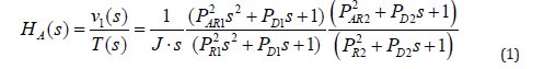
In equation (1):
• J - total moment of inertia.
• P_AR1=1/(2π∙f_AR1), P_AR2=1/(2π∙f_AR2) - the periods of AR frequencies.
• P_R1=1/(2π∙f_R1), P_R2=1/(2π∙f_R2) - the periods of R frequencies.
• P_D1, P_D2 – viscous friction (damping) time constant of first and second resonances.

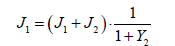
Both resonances are presented as the separate multipliers, where the numerator represents the AR-frequencies and the denominator - the R- frequencies. The lower frequency of first resonance is represented by the first and second stiff coupled bodies (J₁+J₂) that are compliantly linked with stiffness c₂ to the third body with moment of inertia J₃ (Figure 3a). The higher frequency of second resonance is represented by the first and second body moments of inertia only linked with stiffness c₁ while the third body is switched off (Figure 3b).

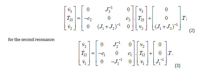
Characteristic polynomials of both models are:

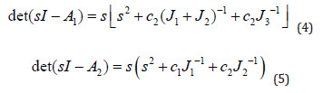
where A₁ and A₂ matrixes are related to the first and second resonance models accordantly.

The transfer function H₁(s) of the motor speed in general form is:

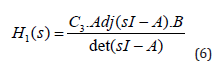
The C₃=[0 0 1] is output matrix for variable v₁, where the transported state matrix for both cases are x₁^T=[v₃ T₂₃ v₂] and x₂^T=[v₂ T₁₂ v₁].

Therefore, the transfer functions H(s) for both resonances are:

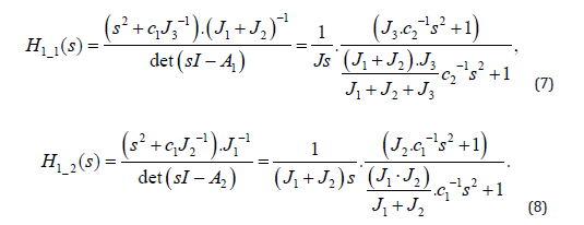
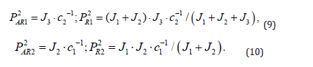
Comparing expressions (7), (8) with (1), a connection between model parameters – the moments of inertia J₁, J₂, J₃ and the couplings stiffness c₁, c₂ to the AR and R resonance’s periods are:

The asymptotical Bode plots for the first body of the model (Figure 2) are presented on Figure 4. The single unit of Bode amplitude slope is equal to 20dB/decade slope.

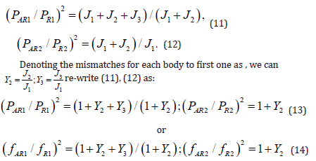
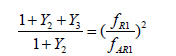
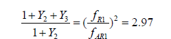
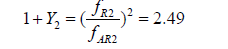
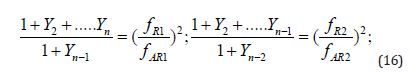
By comparing P_AR1 to P_R1 and P_AR2 to P_R2, we can find the following mismatches:

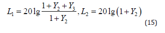
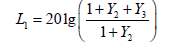
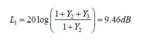
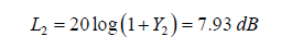
The increments L₁, L₂ of Bode amplitude after each resonance are defined by mismatch ratios for each resonance as follows:

Thus, up to the frequency f_AR1 the Bode slope is determined by the total moment of inertia J=J₁+J₂+J₃, in the range of frequencies f_R1…f_AR2 is determined by sum of moments of inertia (J₁+J₂), and after the frequency f_AR2 is determined only by the 1st body (motor) moment of inertia J₁. Therefore, it could be considered that after each resonance’s frequency one of the bodies is switched off. I.e., the third body is switched off for frequencies higher than the first resonance frequency f_AR1. Due to that fact, it is not considered for the second resonance. Furthermore, the second body is switched off for frequencies higher than the second resonance frequency f_AR2.

Such phenomena with switching off of bodies after resonance leading to Gain increasing which is known as “reduction of effective inertia” [7, 11].

Based on the above, the algorithm of parameter’s’ identification for three bodies’ model may be presented by the following sequence:
1. The total moment of inertia J [kg· m²] of the arm can be calculated with two ways from: transient response or experimental Bode.
• In case of transient response, the total moment of inertia J is can be found as J=T/a, where T is torque at constant acceleration a.
• The total moment of inertia J from experimental Bode

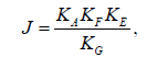
where the total Plant Gain 20logK_G can be found from the Gain Bode at angular frequency of 1rad/s. The Gains of Plant components as current amplifier K_A [Apk/bit], motor torque constant K_T [N· m/ Apk] and position resolution K_E [counts/rad] will be found from the Data Sheets of the motor and the motion controller.

2. First resonance mismatch:

3. Increment L₁:

4. The sum of the first and second moments of inertia with known total moment of inertia J: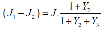

5. Third body moment of inertia:

6. Coupling’s stiffness of the third body:

7. The for the second resonance mismatch with previously calculated sum of the first and second moments of inertia:

8. Increment L₂:

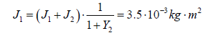
9. The first body moment of inertia (motor’s moment of inertia including stiffer bodies attached to the motor)

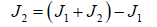
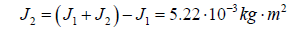
10. The second body moment of inertia:

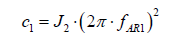
11. The compliant coupling’s stiffness between first and second bodies:

Case study: parameters calculation of robot arm model

The frequency responses of the arm’s Plant (from current amplifier input to axis’ motor speed) - see Figure 1 - were received with Frequency Analyzer build-in modern motion controller [12]. The arm motor speed was detected as first derivation of the motor encoder - rigidly attached to the motor shaft - position.

Initial Data:

• Total moment of inertia J=25.9·10^-3 kg· m²
• Gearbox type: harmonic drive
• AR and R frequencies of the first resonanceR₁: f_AR1 =2.9 Hz; f_R1=5 Hz.
• AR and R frequencies of the second resonance: R₂: f_AR2 =380 Hz; f_R2 =590 Hz

• Calculation of the robot arm model parameters:

1. The mismatch for the first resonance with (J₁+J₂) and J₃ bodies moments of inertia:

2. The amplitude increment L₁:

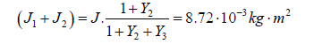
3. The sum of the first and second bodies moments of inertia (J₁+J₂)

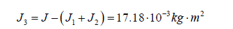
4. The third body moments of inertia J₃

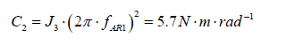
5. The stiffness C₂ between third body coupled and stiff coupled (J₁+J₂) body moment of inertia:

6. The mismatch for the second resonance with J₁ and J₂ bodies’ moments of inertia

7. The amplitude increment L₂:

8. The first body moments of inertia J₁

9. Second body moments of inertia J₂:

10. Stiffness C₁ between second and first bodies

Finally, we can point out that the compliant couplings leading to the resonances of the robot arm are located between:
• The third body with moment of inertia J₃=17.18∙10^-3kg∙m² and stiff coupled bodies (J₁+J₂) =8.72∙10^{-3kg∙m2 are leading to the lower frequency resonance.
• The second body with moment of inertia J₂=5.22∙10-3kg∙m2 and motor with moment of inertia J₁=3.5∙10-3kg∙m2 are leading to the higher frequency resonance.}

Therefore, we can sign out that the source of first lower resonance is the compliance of the robot arm with masses attached on an arm end - for example robot “elbow” arm - and second higher one - the compliance of the harmonic drive gearbox itself.

Using the same approach including the superposition principle and two-body compliant reducer model, a multi-body model can be designed as serially connected n-bodies [13]. These fourth and more bodies should be connected one to the other (Figure 5) using the same principle as the third body shown in Figure 2.

Identification of each resonance will be done by starting from the lowest frequency resonance to the higher ones. The mismatches of this n-body model could be calculated as:

The successively switched off bodies after 1, 2…,(n-1) resonances have the according indexes n,n-1,n-2…,2. Moments of inertia of the bodies with indexes n,n-1,n-2…,2,1 and the coupling’s stiffness n-1,n-2…,2,1 may be found in the sequence using the suggested identification algorithm.

1. Modern motion controllers with built-in frequency analyzers allow for direct receipt of a frequency domain response (Bode) of a robot arm’s plant with the real conditions [14].
2. The key features of the robot arm in the frequency domain are signed out for deep analyses of experimental Bode. And ones will be helpful for understanding the physic process cleanlier.
3. The 2-bodies compliant reducer model can be used to build a robot arm model in the case of 3- and more-bodies as well. Such model could help to understand a structure and identify parameters of most actual cases of n-bodies robot compliant arms.
4. The detection of key compliant couplings allows pinpointing the weakest ones, with a stiff point of view, to improve its stiffness and thus, the performance of robot axes by increasing its servo bandwidth.

None.

No conflict of interest.

1. Bortzov Y, Sokolovsky G (1992) Automatic Electric Drive with Elastic Coupling. St.-Petersburg: Energoatom publishing. In Russian.
2. Gannel L (2017) Identification of multi-body compliant electromechanical actuators. ACS White Paper.
3. Guida D, Nilvetti F, Pappalardo CM (2009). On Parameter Identification of Linear Mechanical Systems. In: third International Conference on CE Applied Mathematics, Simulation, Modeling (ASM'09). Vouliagmeni, Athens, Greece, December pp. 55-60
4. McKelvey T (2000) Frequency domain identification. In 12^th
5. Pintelon R, Schoukens J (2012) System Identification: A Frequency Domain Approach.
6. Schoukens J, Pintelon R, Rolain Y (2004) Time domain identification, frequency domain identification. Equivalencies! Differences? In: Proceeding of the 2004 American Control Conference. Boston, Massachusetts.
7. Ellis G (2001) Cures for Mechanical resonance in Industrial Servo Systems. Proceeding of PCIM. Nuremberg, pp. 187-192.
8. Welch RH and Gannel L (2003) Improving the Dynamic Motion Behavior of a Servo System with Low Mechanical Stiffness. In: 38^th Annual meeting of IEEE Industry Application Society. Salt Lake City, USA.
9. Gannel L (2017) Defining the compliance of electromechanical linear actuators. Design World, August: 56-61.
10. Gudzenko A, Gannel L and Smotrov E (1987) The synthesis of modal control in high bandwidth transistor's electric drives. Electricity 1: 40-46.
11. Gannel L (2013) Built-In Filters to Suppress Vibrations in a Linear Elastic Electric Drive on Account of Reduction in the Effective Mass. Russian Electrical Engineering 84(3): 145-148.
12. Formalskii A, Gannel L (2015) Control to Avoid Vibrations in Systems with Compliant Elements. Journal of Vibration and Control 21(14): 2852-2865.
13. Juang JN (1994) Applied System Identification. New Jersey: Prentice Hall.