Comparative Study of Linear Kernel and Gaussian Kernel in Gaussian Process Regression

Machine learning [1, 2] is the core of artificial intelligence. Its main idea is to use the existing data that has been mastered, analyze and process the data, and seek rules from it. Finally, predict the unknown through the analysis of known data, and the most critical one is machine learning algorithm. In recent years, Gaussian process [3,4,5] has attracted wide attention due to its effectiveness. Gaussian process is an effective machine learning method [6,7], which combines both Bayesian theory and kernel theory, and thus has the advantages of both machine learning methods. Gaussian process can realize both classification and regression [7], which has certain advantages. Gaussian process model [8,9], as an excellent machine learning model in the field of regression and classification, has been widely concerned, and many excellent successes have been born at the right moment. Gaussian process has a lot of applications in practi cal problems [10,11]. The second part describes the process from unary Gaussian distribution to multivariate Gaussian distribution and then to Gaussian, and introduces the kernel function used in this paper. The third part strictly deduces the Gauss process regression model.

The fourth part is the experimental part of the algorithm. Three evaluation criteria are used to analyze the performance of the model with different kernel functions, and the results are obtained.

Gaussion distribution

The simplest and most common unary Gaussian distribution [12], the probability density function is

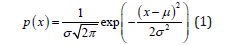
μ is mean and σ is variance, and the probability density function is drawn as the familiar bell curve. From unary Gaussian distribution to multivariate Gaussian distribution [13] [14], it is assumed that each dimension is independent of each other

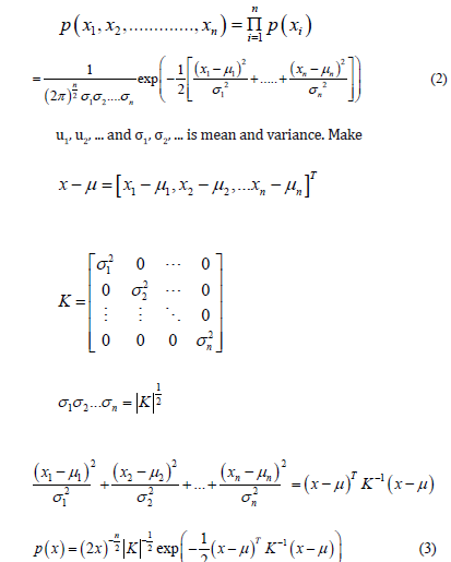
Where μ ∈ n is the mean vector, and K ∈ n×n is the covariance matrix. Since we assume that each dimension is directly independent of each other, K is a diagonal matrix. When variables of each imension are correlated, the form of the above equation is still the same, but in this case, the covariance matrix K is no longer a diagonal matrix and only has the properties of semi-positive definite and symmetric. This is also commonly abbreviated as

Therefore,A mean and a variance determine a onedimensional Gaussian distribution, and a mean vector and a covariance matrix determine a multidimensional Gaussian distribution

Gaussion Process

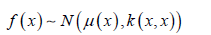
When we look at sampling from the perspective of function and understand that each sampling with infinite dimension is equivalent to sampling a function, the original probability density function is no longer a distribution of points, but a distribution of functions. This infinite element Gaussian distribution is called a Gaussian process. Gaussian processes are formally defined as: for all

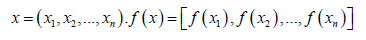
all obey the multi-element Gaussian distribution, Then f is said to be a Gaussian process, expressed as

The μ ( x) ∈ n →n indicates the Mean function and returns the mean of each dimension; The κ ( x, x): n ×n →n×n is a covariance function Covariance Function (also known as the Kernel). Function returns the ovariance matrix between the dimensions of two vectors. A Gaussian process is uniquely defined as a mean function and a covariance function, and subsets of the finite dimensions of a Gaussian process all obey a multivariate Gaussian distribution (for ease of understanding, we can imagine a binary Gaussian distribution in which each dimension obeys a Gaussian distribution).A Gaussian process can be determined by a mean function and a covariance function!

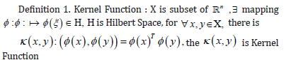
kernel Function

The kernel takes the vectors in the original space as input vectors and returns the function of the dot product of the vectors in the feature space (converted data space, possibly higher dimensional) [15,16].

Linear kernel
Computes a covariance matrix based on the Linear kernel between inputs X₁ and X₂ :

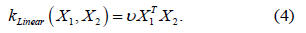
where - v is a variance parameter.
RBF
Computes a covariance matrix based on the RBF (squared exponential) kernel between inputs X₁ and X₂ :

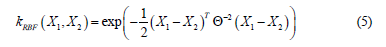
where Θ is a lengthscale parameter. See gpytorch. kernels. Kernel for descriptions of the lengthscale options.

GPR

The formula of Gaussian process regression is derived as follows. Gaussian process a priori said

This is a prior distribution representing the output y we expect to get after input x before looking at any data.
After that, we import some training data with input x and output y = f (x) .Next, we have some new input x* and need to compute y* = f ( x* )

If now we observe some data (x*, y* ) and assume that y* and f(x) obey joint Gaussian distribution

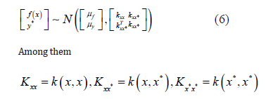
Have x, y as the training data, x* for the input data), now, the model is p (Y* X *, X ,Y ),What we need is *

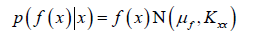
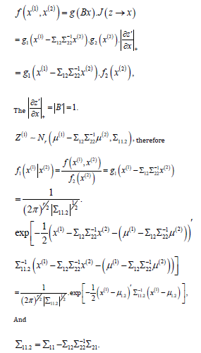
This becomes a given joint Gaussian distribution, finding the conditional probability P(y* x*, x, y):

The above formula indicates that the distribution f of the function after given data (x∗, y∗) is still a Gaussian process. The specific derivation is as follows:

Here are some definitions and theorems:

Definition 2. Set for random vector, 1,... q U U ,Uqare independent of each other and with

N(0,1) distribution; Let μ be p dimensional constant vector and A be p×q constant matrix, then the distribution of X = AU +μ is called p dimensional normal distribution or X is called p dimensional normal random vector. Write it as .

Say simply, by q a independent standard normal random variable of some linear group of the distribution of the random vector, is referred to as multiple normal distributed.

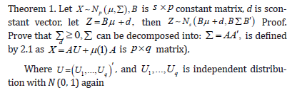
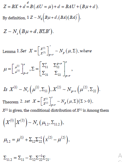
Proof. Prove that for a nonsingular linear transformation, let

So theorem 3.4 tells us that

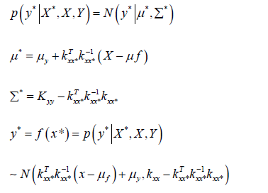
This is the posterior distribution of y∗ calculated based on the prior distribution and the observations. In the case of GPR, this formula helps us get the predicted value, and in most cases u = 0

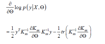
Marginal maximum likelihood (MLL)

These are modules to compute the marginal log likelihood (MLL) of the GP model when applied to data [17,18,19]. I.e., given a GP f G(μ,K), and data X, y, these modules compute

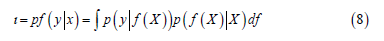
This is computed exactly when the GP inference is computed exactly . It is approximated for GP models that use approximate inference.
These models are typically used as the ”loss” functions for GP models (though note that the output of these functions must be negated for optimization).
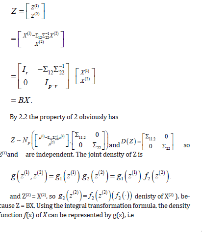
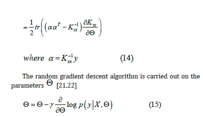
From 2.2 ,we know that:

Therefore, the optimized parameter model can be obtained [20] (take RBF kernel function as an example).

Dataset

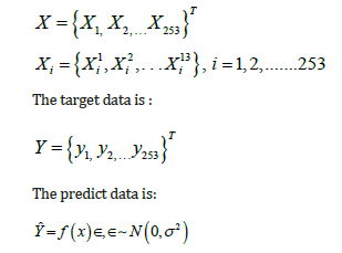
The data set contains information about housing prices in Boston, Massachusetts collected by the U.S. Census Bureau. The data set contains 506 samples.It contains 13 characteristic variables and a target value: the average house price.Below is a brief introduction to the housing price data setGaussian process regression was performed on the above Boston housing price data set, and the dataset was randomly divided into a training set and a test set in a 1:1. We assume that the data of the training set obey the Gaussian process, so as to predict the average housing price (Figure 1).

GPR Algorithm

According to the Dataset, we can get the input training data as follows:

The training set was trained for 5 epochs, every epoch was iterated 1000 times, and the MLL function was used to calculate the loss of the predicted value and the target value. Fig 2 shows the loss function image of the model against the training data set after Gaussian process regression uses linear kernel function and RBF kernel function respectively.

As can be seen from the figure, the loss function value of the model using linear kernel function is lower than that using RBF kernel function in the same training batch, and the rate of decline is faster. When the loss function converges, the loss value of the model using linear kernel function is lower than that using RBF kernel function. Therefore, from the convergence of loss function, the model using linear kernel function performs better. Table 1 and Table 2 show the partial parameter values of the model in the training process (Table 1,2 & Figure 2).

Table 1:Parameter.

Table 1:Parameter.

Fig 3 and Fig 4 respectively show the fitting between the predicted value and the real value of the Gaussian process regression model under the two kernel functions. The comparison between FIG. 3 and FIG. 4 shows that the predicted value of the model under the linear kernel function better fits the original real value. Therefore, in terms of the fitting of the predicted value, the model using linear kernel function is better than that using RBF kernel function.

Metric

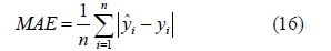
The evaluation criteria of three regression models are used in this paper. Mean Absolute Error(MAE): Is the average value of absolute error, which can better reflect the actual situation of predicted error.

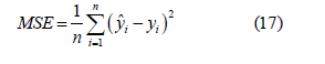
Mean Square Error(MSE):Is the square of the difference between the predicted value and the true value, and then the average of the sum, generally used to detect the deviation between the predicted value and the true value of the model.

R2 squared:Coefficient of determination. Reflects the accuracy of model fitting data, generally R2 range is 0 to 1. The closer the value is to 1, it indicates that the variable of the equation has a stronger ability to explain y, and this model also fits the data well (Figure 3).

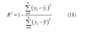
Fig 5 shows the MAE value of the Gaussian process regression model on the test set under the two kernel functions. MAE values for partial iterations are listed in the table. As can be seen from Figure 5, MAE under the linear kernel model is much smaller than that under the RBF kernel model. It can be seen that, from the perspective of MAE evaluation criteria, the model using linear kernel function has better performance than that using RBF kernel function (Figure 4).

The value of MSE is shown in Figure 6. As can be seen from the figure, the mean square error using the linear kernel model is smaller, which means that the predicted value using the linear kernel model has less deviation from the real value. Therefore, from the point of view of mean square error, it can be seen that the advantage of using linear kernel function is more obvious (Figure 5,6).

Figure 6 shows the value of R2square. It can be seen from the figure that the R2square value of the model using linear kernel function is closer to 1 than that of the model using RBF kernel function. The closer it is to 1, the stronger the interpretation ability of the model to the real value is, thus indicating the better fitting degree of the model to the data. So in this respect you can also see the advantage of using linear kernel functions.

Gaussian process regression can effectively simulate data, but the choice of kernel function has a great impact on the simulation results of data, so how to choose a suitable kernel function when we use Gaussian regression model becomes very important.In this paper, the linear kernel and RBF kernel are compared in the Gaussian process regression model, and it is concluded that the linear kernel is better than RBF kernel in this data set. Therefore, we know that the selection of kernel function should not only consider the efficiency of its own model, but also consider the influence of data set itself. Therefore, in the future work, I hope to find a better and faster method to select the kernel function more suitable for the model, so as to achieve a better prediction effect on the data.

“Supported by: Fundamental Research Program of Shanxi Province Fund number: 202103021223379” to the article.

No conflicts of interest.

1. JR Quinlan (1993) Program for machine learning.
2. C Andrieu, ND Freitas, A Doucet, MI Jordan (2003) An introduction to mcmc for machine learning. Machine Learning 50(1): 5-43.
3. D Nguyen-Tuong, J Peters (2008) Local gaussian process regression for real-time model-based robot control. In Intelligent Robots and Systems.
4. A Girard, CE Rasmussen, R Murray-Smith (2002) Gaussian process priors with uncertain inputs - multiple-step-ahead prediction. School of Computing Science.
5. AJ Smola, P Bartlett (2000) Sparse greedy gaussian process regression. In Neural Information Processing Systems.
6. H Owhadi, JL Akian, L Bonnet (2022) Learning “best” kernels from data in gaussian process regression. with application to aerodynamics. Journal of Computational Physics.
7. CE Rasmussen, Cki Williams (2006) Gaussian processes for machine learning (adaptive computation and machine learning). The MIT Press.
8. Joaquin, onero Candela, CE Rasmussen (2005) A unifying view of sparse approximate gaussian process regression. The Journal of Machine Learning Research 6: 1939-1959.
9. M Seeger, Cki Williams, ND Lawrence (2003) Fast forward selection to speed up sparse gaussian process regression. In International Conference on Artificial Intelligence and Statistics: 254-261.
10. B Lu, D Gu, H Hu, K Mcdonald-Maier (2012) Sparse gaussian process for spatial function estimation with mobile sensor networks. In Emerging Security Technologies (EST). Third International Conference on.
11. O Stegle, SV Fallert, DJC Mackay, S Brage (2008) Gaussian process robust regression for noisy heart rate data. IEEE transactions on bio-medical engineering 55(9): 2143-2151.
12. Govind S Mudholkar, Ziji Yu, Saria S Awadalla (2015) The mode-centric m-gaussian distribution: A model for right skewed data. Statistics & Probability Letters 107: 1-10.
13. Stein, M Charles (1981) Estimation of the meaning of a multivariate normal distribution. Annals of Statistics 9(6): 1135-1151.
14. C Stein (1956) Inadmissibility of the usual estimator for the mean of a multivariate normal distribution. University of California Press: 197-206.
15. S Bergman (1950) The kernel function and conformal mapping. American Mathematical Society.
16. P Li, S Xu (2005) Support vector machine and kernel function characteristic analysis in pattern recognition. Computer Engineering and Design.
17. BM Aitkin (1981) Marginal maximum likelihood estimation of item parameters: Application of an em algorithm. Psychometrika 46: 443–459.
18. JL Foulley, MS Cristobal, D Gianola, S Im (1992) Marginal likelihood and bayesian approaches to the analysis of heterogeneous residual variances in mixed linear gaussian models. Computational Statistics & Data Analysis 13(3): 291-305.
19. P Kontkanen, P Myllymaki, H Tirri (2013) Classifier learning with supervised marginal likelihood. Morgan Kaufmann Publishers Inc: 277-284.
20. Y Bazi, F Melgani (2009) Gaussian process approach to remote sensing image classification. IEEE Transactions on Geoscience and Remote Sensing 48(1): 186-197.
21. YX Hao, YR Sun, SO Sciences (2018) Knearest neighbor matrix factorization for recommender systems. Journal of Chinese Computer Systems.
22. YX Hao, J H Shi (2022) Jointly recommendation algorithm of knn matrix factorization with weights. Journal of Electrical Engineering & Technology 17: 3507-3514.