A Very Small Radio Telescope Array

Hydrogen is the most abundant element in the Universe, making up 80% of the total mass (the rest being mostly helium). Such hydrogen formed soon after the big bang and, as the Universe expanded and cooled, volumes of hydrogen clumped together to form clouds that shuddered into smaller clouds to form the galaxies. Thus, our galaxy, the Milky Way, is mostly a collection of neutral hydrogen. The hydrogen atom can exist in two ground states, one where the spin of the proton and electron are parallel, and the other (of less energy) where they are anti-parallel. A hydrogen atom can exist for up to 11 million years on the upper state before settling on the lower state of anti-parallel spin. When an atom falls to the lower state the difference in energy is emitted as a photon (Figure 1) with a wavelength of λ = 21 cm. Knowing that c = λν, the emission must occur at 1,420 MHz; this process is so rare that it has never been observed in a laboratory.

The possible detection of the 21 cm line of hydrogen was proposed in 1944 by Christof Henryk van de Hulstin of the Leiden Observatory during a meeting of the Nederlands Astronomen Club to discuss the pioneering work of Jansky and Reber. On the face of it, the hyperfine transition scarcely seemed a hopeful proposition because i) the temperature of interstellar atomic hydrogen would be very low, ii) the hyperfine transition probability only about once in millions of years, and iii) the density of hydrogen would not average more than about 1 atom per cubic centimeter.

Fortunately, the vast extent of the Galaxy compensates for these discouraging factors, and van de Hulst suggested the search, however, because of World War II, the discovery of the 21 cm line of hydrogen would have to wait. In 1951, three different research groups, namely Oort and Muller in the Netherlands, Ewen and Purcell at Harvard, and Christiansen and Hindman in Australia all detected the 21 cm line within a few weeks of each other, and reported their findings in the same edition of Nature. As had been foreseen, the prediction of the 21 cm line proved to be of great fundamental importance, a basic step in establishing a valuable method of studying the structure of the galaxy. Since the hydrogen in the Milky Way is moving in clouds with respect to the solar system, a Doppler shift of the 1,420 Mhz frequency will appear. Indeed, the frequency will shorten when the clouds move towards the solar system, and lengthen when they move away from us. Since the relative movement is non-relativistic, a simple formula can yield the velocity component that the cloud moves along the line on sight of the array:

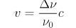
With this calculation a simple distribution of the radial velocities of hydrogen can be generated, this information is necessary for modeling the structure of the Milky Way.

Sidereal Time (ST) is a measure of which meridian of the celestial sphere is passing the local meridian of an observing location, a sidereal day is just under four minutes shorter than a regular solar day, this is due to the displacement of the earth in its orbit with relation to stars, see Figure 2. In the calculation of Sidereal Time, the calculation of the Julian century (T) is necessary.

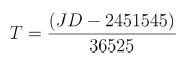
where JD is the Julian Day discussed below. The formula for Sidereal Time is:

To calculate the exact Sidereal Time at the observing location, the Julian Day (JD), a number that is independent of the day of the week, month or year, must be calculated as follows:
A = −Int(7 ∗ ((Month + 9)/12 + Y ear)/4)
B = Sgn(Month − 9)
C = Abs(Month − 9)
D = Int(Year + B ∗ Int(C/7))
E = −Int((Int(D/100) + 1) ∗ 3/4)
F = A + Int(275 ∗ Month/9) + E + Day
JD = F + 1721027 + 2.5 + 367 ∗ Y ear

Where Day, Month and Year correspond to the regular calendar day of observation. Here, the functions Int() gives the Integer part of the expression, Sgn() returns the sign of the expression and Abs() returns the absolute value of its argument. This system (Figure 3) defines Altitude (h) as the degrees of elevation from the Horizon up 900 at the Zenith or highest part of the sky in the observing location. Azimuth (A) is measured along the horizon in degrees, 360 being the full circumference. Although Azimuth is measured from the North in a clockwise manner. In astronomy it is usually measured from the South also in a clockwise manner, this project uses the latter. An object in the sky will have constantly changing Altazimuthal coordinates due to the Earth’s rotation.

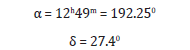
This coordinate system represents a projection of the Earth’s rotation in space onto the celestial sphere. The North and South Celestial Poles correspond to the poles where the Earth rotates. Perpendicular to these poles is the celestial equator, which is divided in 24 segments or hours. The division of the equator, called Right Ascension, is denoted by α. Declination, the degrees from the equator to the celestial poles, is designated by δ (Figure 4). Hour angle is the difference of an object’s Right Ascension and the local Sidereal Time, it is calculated by H = θ − α or H = θ₀ − L − α where θ₀ is the sidereal time at Greenwich and L the observer’s longitude (positive west, negative east from Greenwich). The galactic coordinates are a system of coordinates used to measure locations of the celestial sphere using our galaxy as a reference (this system of coordinates will be the one primarily used by the project). Its principal circle is the milky way, defined as the galactic equator, divided in 3600 to define galactic longitude (l), perpendicular to the galactic equator are the North and South Galactic poles, the 900 required to reach the galactic poles from the equator is referred to as galactic latitude (b). The origin for the galactic longitude was defined by the International Astronomical Union in 1959. In the equatorial system of B1950.0, the location of the galactic (Milky Way) North Pole has the coordinates

The origin of the galactic longitudes is the point (in western Sagittarius) of the galactic equator which is 330 distant from the ascending node (in western Aquila) of the galactic equator with the equator of B1950.0. These values have been fixed conventionally and therefore must be considered as exact for the mentioned equinox of B1950.0 (Figure 5).

Since the antennas are parabolic, all incoming waves are reflected to a same location, called focal point. Its location can be calculated from the center of the antenna to it. This distance is called focal distance and can be calculated by F = D/4, where D is the diameter of the antenna. The directivity of a parabolic reflector is proportional to the aperture radius a and the aperture efficiency E.

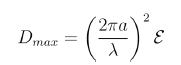
Where a typical value for the efficiency is 55%. The antenna Half-Power Beam Width is approximated by the formula

Where a is the aperture radius. In this case a=152.4 cm, so

The value is small because of the high frequency of observation, it can be seen that as the frequency drops the wavelength increases, therefore increasing Half Power Beam Width.

The geographical coordinates used for the location of the array are described in Table 1. The actual antennas used are presented in Figure 6, and schematics of the diagram used is in Figure 7. The Earth’s geographical North and Magnetic North do not match, so for every location a compass will only yield and apparent direction of the actual geographical North, there will be a certain displacement either West or East for true North, such displacement is called Magnetic Declination, it varies for different locations on the planet. The magnetic declination used to obtain true north location was 90 and 49m West (Source: USGS.) The maximum separation possible between the antennas is 34 meters, due to the orientation of the building (Table 1).

Table 1:Geographical Coordinates of Array

The unit used for detection is commercially available, two modes of operation are possible, Continuum mode, which monitors only a frequency of 1,420 MHz and Spectrum mode, which sweeps a spectrum of 1,200 KHz wide centered at 1,420 MHz (600 KHz in each direction). This second mode is the one used to obtain images of the passing of the milky way in front of the array, the first mode can be used in calibrating the actual passing of the milky way on the antenna’s line of sight against the predicted times of this event by the program. The antennas used are 10 ft parabolic dishes commercially used for satellite TV reception which were very common 10 to 15 years ago, since most people have migrated to new smaller dishes, most have been discarded by owners. The pair used were donated by local area residents but the mesh had to be repaired on one of them (the antenna itself had been lying on the ground as scrap metal for nearly ten years). Since the original mesh is no longer available, a suitable mesh had to be found, the only restrictions were that the mesh separation had to be smaller than the wavelength to be observed (21 cm) and be malleable enough to bend into a parabolic curvature, fortunately such materials are still available. The Low Noise Amplifier (LNA) units provide 26 dB of gain, since the measured signal is very high in frequency, the gain is necessary to transport it to from the antennas to the spectrometer, one of them was placed directly at the feedhorn and the other one along the line before both signals were combined. The Cable used is specification RG-8, which is commercially used for communications applications, the available loss charts did not go up to the frequency used (1,420 MHz), so a rough approximation was approximated from the attenuation charts, yielding 20 dB per 100 ft. The different sections of cable used must be properly connected to avoid radiation ingress from the Sun and must be also sealed against humidity, both circumstances can hamper or obliterate the quality of the signal [1].

The code for this program comes mainly from the one developed at Stephen F. Austin University [2], this program records the signal levels of the 1200 KHz spectrum centered at 1,420 MHz and the local time of observation. It has been modified so that the observations record the intensity of the signal, local time, and the current sidereal time and galactic coordinates at observation. This requires additional input before an observing run, such as the observing location’s geographical location, time zone with respect to Greenwich and the altazimuthal coordinates that the array will be pointing at. This program was developed independently but it has been mostly included as an addition to the Data Collector program, however its standalone version provides the times at which the Milky Way will pass in front of the array’s observing direction, the required inputs are the ones just described as the additions to the data collector in the previous section. This program takes the data files created by the Data Collector software and creates an image of the intensity of the observed voltages during the observation run. It assumes a Gaussian distribution of the recorded signals and assigns a color coding to it. Additionally, it creates graphs of the mean difference of the voltage readings and the change in galactic latitude during the time duration of the data file.

The Data plotter first computes the average (or mean) of the voltages for the entire file, it looks for the maximum and minimum values and calculates the standard deviation of the data. Color assignments are done by selecting a dividing line, called scale, measured in units of the standard deviation away from the mean of the voltages. Anything to the left is assigned black, and the rest to the right will be divided into seven even color zones. The original scale line in the data plotter program is set to one standard deviation, thus everything to the left of one standard deviation to the right of the mean will be assigned black and the rest of the data will be divided into seven colors (white representing highest intensity. Additionally, a calculation of the histogram of the data points has been included as a form of checking that the distribution of the signal does follow a Gaussian distribution, if it does not (in the case of saturation) a check box is included in order to filter the unwanted levels.

The first image produced (Figure 8) was that of the feedhorn connected directly to the spectrometer, the antennas were not repaired yet, the 24-hour scan was also done indoors. No significant image was obtained until the first antenna was repaired and set up on the roof of the physics building, the base was not ready, so it was just left on the floor pointing to the zenith. The obtained image, Figure 9, clearly shows the passage of the Milky Way on two occasions.

For the March 11 image, the times when the maximum signals were detected were 9:25:10AM and 6:28:23PM, the signal levels where graphed along with the signal at the time in between both readings (Figure 10). To verify that those times represent the moment when the Milky Way was crossing in front of the antenna the following images (Figures 11&12), obtained from a Planetarium simulator, represent the sky’s position in the direction that the antenna was aimed (Zenith).

Table 2:Observation Results.

Table 3:Velocity Calculations.

The results for this reading are described in Table 2, following the formula for the velocity of the Milky Way observed on those occasions is in Table 3.

The graphs that were produced from the previous data run (March 11) were analyzed and are presented in Figure 13. The top one represents the average voltage over the duration of the 24- hour run, on this one it is difficult to ascertain when the Milky Way crossings occurred, since their presence of random noise makes the possibility of detection much harder. The second graph of Figure 13 represents a difference between the general mean and the mean of the positive Doppler shift and the mean of the negative Doppler shift of the observed spectrum. As can be seen when the Milky Way is not present, the graph represents a flat line and peaks up or down depending on whether the positive or negative Doppler shifts dominate the spectrum readings. In order to track random noise in the environment, the bottom graph of Figure 13 of only the base frequency of 1420 Mhz was produced, resembling the top average voltage graph. The presence of the sun during daytime observation is of no consequence during the spring and winter months, however the LNA’s become too hot in the summer months which induce thermal noise, shadowing and in some cases overcoming any detectable signal. The level at the spectrometer saturates to its maximum value, introducing excessively high readings in the recorded file, which yield an erroneous output image.

The preceding work has shown how the advancements of technology allows institutions to reproduce the detection a fundamental emission in astrophysics that took 5 years to be shown in existence after it was postulated. 50 years ago, computers were not easily available and it took the use of massive and expensive equipment to detect radio sources. In some of the literature from the bibliography the need for an entire building to house the detection. In order to obtain better resolution in the obtained images, more antennas will be needed, and as a recommendation the possibility of moving the array to a new location should be considered, also the newer antennas could be placed on the roofs of other departments and a communications link could be established, the possibility of it being wireless should also be looked at. Figure 14 shows the application used for data capture. A university in the southern hemisphere that makes these observations should be contacted or encouraged to set up an array, this way observations from both hemispheres can be compiled and the entire milky way can be mapped, this combined data could be used to create a rough model of the milky way following the Oort model described in [8]. The web site of this project is https://utminers.utep.edu/lbasurto3/.

• Berni Alder, Sidney Fernbach, Manuel Rotenberg (Editors) (1975), Methods in Computational Physics. Volume 14, Radio Astronomy, Academic Press.
• Dan Bruton, Web Page of the Stephen F. Austin University, Radio Observatory, Nacogdoches, TX, USA.
• Burke B, Smith F Graham (2002) An Introduction to Radio Astronomy, Cambridge University Press.
• Goldsmith Paul F (Editor) (1988) Instrumentation and Techniques for Radio Astronomy, IEEE Press.
• Hey JS (1971) The Radio Universe, Pergamon Press.
• Hey JS (1973) The Evolution of Radio Astronomy, Elek Science.
• Karttunen H, Kroger P, Oja H, Poutanen M, Donner KJ (2003) Fundamental Astronomy, Springer-Verlag.
• John D Kraus (1986) Radio Astronomy, Quasar-Cygnus Books.
• Bernard Lovell, Joyce Lovell (1963) Discovering the Universe, Harper & Row.
• McKelvy M, Spotts J, Siler B (1997) Using Visual Basic 5, QUE.
• Jean Meeus (2000) Astronomical Algorithms, Willmann-Bell Inc.
• Piddington JH (1961) Radio Astronomy, Harper & Brothers.
• George B Rybicki, Alan P Lightman (1985) Radiative processes in Astrpophysics, Wiley-Interscience.
• Frank H Shu (1982) Physical Universe: An Introduction to Astronomy, Univeristy Science Books.
• Richard Thompson, James M Moran, George W Swenson Jr (Editors) (2001) Interferometry and Synthesis in Radio Astronomy, John Wiley & Sons Inc.
• Gerrit L Verschur (1974) The Invisible Universe Revealed: The Story of Radio Astronomy, Springer-Verlag.
• Fiona Vincent, Positional Astronomy.
• Lodewijk Woltjer (1966) Galaxies and the Universe, Columbia University Press.