Modeling and Optimization of The Energy Bill

The economic evolution of Companies is clocked by their energy strategies in terms of raw materials and processes coupled with a wide variety of national regulations on energy and environmental policy adopted by the company. The relationship between global economic developments and decisions in the energy sector is critical. The weight of the energy bill, the influence of level of activity on energy consumption, or conversely the effect of energy investments on the overall activity are sensitive, as well as their consequences for growth, employment and inflation. The formalization of this relationship is complex for reasons relating to the specificity of energy production and difficulties to forecast the long-term demand. Mathematical modeling is the art of representing a physical reality in abstract models accessible to analysis and calculation. Much of applied mathematics is, in some way, to do modeling, define one (or several) model (s), mathematics, for reporting of a sufficiently general, a given phenomenon to identify one (or more) mathematical model [1]. There are many methods of statistical modeling. We only process the basic linear model (Gaussian). In the method described, there is almost always a special variable called generally dependent variable, or response variable, and denoted Y (this is a random variable). The goal is then to model a variable Y depending on variables observed on the same sample X.

The Principal Component Analysis (PCA) is part of the data analysis, which is to reduce the number of descriptive characters and seeking the most faithful projection plane by distorting the least possible reality. The characters obtained through this analysis are new characters ‘principal’ [2]. Predicting the future is all about optimizing decisions must be based on an increasing number of data [3]. It is not easy to handle this data in hand it is the reason for which data processing software is used. In our study we used the SPSS statistical analysis software.

Modelling of the principal component’s analysis

The descriptive analysis: In the first place we start with descriptive statistics (mean, standard deviation ....). The table below represents the various elements of the descriptive analysis:

According to the above table the sulfur consumed average is 4790.02 T with a standard deviation of 449.078 T which means that the average is significant enough, it means that the majority of observations are very close to the average (the values are not too dispersed around the average). For steam HP, MP, and EE H₂SO₄, however for the consumption of sea water from an average of 616,090.61 and a standard deviation of 58,755.744 shows that the values are dispersed around the average.

Correlations table: We then study the correlation between the different variables. The table 2 represents the correlations between the various input-output sulfuric plants. This is the correlation matrix that gives an insight into the relationship between pairwise variables. Note that all correlations are positive (all variables vary in the same direction) which means that characters are considered correlated. There are strong positive correlations around 0.987 and 0.828 respectively between HP steam, MP steam and sulfuric acid production, which explain the influence of H2SO4 production on HP and PM steam production and thus the power generation platform. A strong positive correlation in the order of 0.816 between steam extraction and steam HP production which explains why it has less losses in steam extraction.

Table 1: Descriptive statistics.

Table 2: The correlation between the different variables.

It is also noted that there is a very high correlation between the consumed sulfur and sulfuric acid product it indicates that, for a good combustion and conversion absorption generates good production of sulfuric acid and vice versa. On the other hand, we cannot estimate a correlation between the production of MP steam and the seawater consumption since our correlation coefficient is not sufficiently determinative which is of the order of 0.482.

Factorial analysis: The projection of variables on a plane gives the distribution shown in the following diagram.

Linear regression

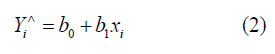
A regression problem is to find a function f such that for all i, Yi is approximately equal to f(Xi). The simplest case is that of simple linear regression. In simple linear regression, it is to estimate the parameters and test the validity of the model [4,5].

With: b₀ is the intercept: The value of Y when X = 0.

b₁ is the slope: variation caused by the variation of one unit of X.

e_i is a random variable reflecting the inadequacy of the model.

We will estimate the β vector by a vector b. There will therefore be a straight:

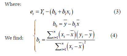
To estimate we use the famous method of least squares [6], which is to choose b₁ and b₀ therefore the sum of the squared differences ei between the observed values and calculated values is minimum.

The term that minimizes,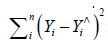

We measure the adequacy of the estimated regression equation to the observed values yi by R² “coefficient of determination” [7]:

R² expresses the percentage of the sum of total l square “explained ‘by the estimated regression equation.

With:

In our study we want to investigate the influence of the sulfur consumption in thermal power (HP steam), Indeed we wanted to know how to predict it from the quantity of sulfur consumed. To do this, we opted for the simple linear regression from data provided by the platform. This database includes various input-output sulfuric workshop.

Variable introduced/ removed: The Table 3, expresses the variables that have been introduced into the model, the two variables (dependent and independent) were included in the model, since we use a simple regression.

Table 3: The variables introduced into the model.

Model summary: On the summary table of the model below, SPSS calculary coefficient de correlation R quiets comprise entre -1, 1, which also represents the percentage of the variance (thermal energy) for the variable (consumed sulfur). It should be noted that a good linear fit involves R close to 1. In our case the value of the R correlation coefficient is 0.986, which is very significant if we raise to the square this coefficient we get the determination coefficient that determines how the regression equation is adapted to explain the distribution of points is about 0.972 confirming that the independent variable (consumed sulfur) influence on the independent variable (HP steam) and in this case steam production can be predicted from the consumption of the sulfur.

The model parameters: The last table gives us the model parameters and their degrees of significance.

From the table above, we can write:

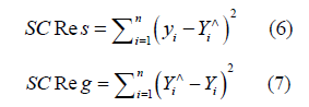
Table 4 allows us to identify non-standardized coefficients that allow to know the way of relationship between the predictor and the dependent value. In our study the intercept is B = 942.773 and the slope indicated by the B value for the independent variable sulfur consumed. And also, the standardized coefficients Beta (β ), which reflects the value that an independent explanatory weight can have on the dependent value.

Table 4: The model parameters and their degrees of significance.

The maximum energy efficiency, a fundamental challenge for sustainability of production, suggests solutions for the mastery of electricity consumption. In our case, modeling and optimization of the energy bill was necessary. Indeed, thanks to the ACP method, synthesized and summarized data, we could highlight trends combinations or contrasts between individuals or between variables. Information obtained via the graphical representations and correlations table allowed us to choose the model of simple linear regression to study the connections of the energy cycle of the workshop between the sulfur consumed and HP steam produced to address the problem of energy modeling, first step towards optimizing energy bills. This modeling allowed HP steam management and thereafter, developing the energy performance of the thermal station used for the production of electrical energy.

None.

No conflict of interest.

1. Philippe Besse (2003) Pratique de la modélisation statistique. Publ Lab Stat Probab Univ Paul Sabatier Toulouse Dispon, Partir L’URL Httpwww-Sv Cict FrlspBesse.
2. JLL Moigne (1994) La théorie du système général: théorie de la modélisation. jeanlouis le moigne-ae mcx.
3. Jean-Marie Bouroche, Gilbert Saporta (1987) L’Analyse des donné Presses Universitaires de France - PUF.
4. George AF Seber, Alan J Lee (2012) Linear Regression Analysis. John Wiley & Sons.
5. Sylvie Huet, Emmanuel Jolivet, Antoine Messéan (1992) La régression non-linéaire: méthodes, applications en biologie. Editions Quae.
6. P Tchébychev (1859) Sur l’interpolation par la méthode des moindres carré Eggers, Comp.
7. JS Tanaka, GJ Huba (1989) A general coefficient of determination for covariance structure models under arbitrary GLS estimation. Br J Math Stat Psychol 42(2): 233‑