Enhancing Predictive Models for Longitudinal Welding Distortion in Thin Plates

Introduction

Welding is widely used in various industries, but it unavoidably leads to the creation of residual stress and distortion. This occurs primarily because the metal goes through non-uniform expansion and contraction as it repeatedly heats up and cools down during the welding process. These consequences can have substantial impacts on factors such as structural strength, fatigue life, localized strain patterns, and the integrity of the welded surface [1-3]. It’s essential to grasp the extent of these residual effects when designing steel structures. In the pursuit of this understanding, Hibbitt and Marcal [4] took an initial step by using the finite element method to forecast the residual stresses induced by welding. Their study involved modeling a circular weld on a symmetrical disc. The results obtained from their thermal model demonstrated a strong alignment with experimental data, although it’s worth noting that only the maximum stress value matched the measurements conducted in the laboratory. Ma et al. [5] investigated the impact of plate thickness, intermittent support conditions, inlet temperature, and the number of welding passes on the residual stresses and distortion generated during welding. They utilized 3D finite element modeling as their approach to delve into these aspects. Tsui et al. [6] as well as Bolshakov et al. [7] researched to investigate how residual stress affects hardness and elastic modulus. They accomplished this by conducting conical indentation experiments and utilizing finite element analysis (FEA). Their results pointed to a correlation between hardness and elastic modulus with residual stress when con sidering the theoretical contact area based on indentation displacement. However, this relationship vanished when accounting for the actual contact area. In a different study, Michaleris and DeBiccari [8] investigated the influence of the modeling approach on predicting welding-induced distortion. They also explored the impacts of factors such as sheet thickness, the presence of hardeners, and the spacing between hardeners using finite element analysis.

Andersen et al. [9,10] developed a finite element model specifically for welding steel sheets. Their model accounts for important variables such as welding speed and input heat as significant factors in the simulation. Their research findings indicated that welding speed, input energy, and heat source distribution have a significant influence on the results and outcomes of the welding process [11-20]. The speed of welding affects the deformation or shape change of the material, while the input energy has an impact on the boundaries of the fusion zone and the distribution of heat. Precisely controlling these factors is essential for achieving the desired weld quality and effectively managing the heat-affected zone. In a study by Long et al. [21], they examined the residual stress and distortion that occur during butt welding. Their research concluded that both the thickness of the sample and the welding speed significantly impact the magnitude of residual stress and distortion generated by the welding process. Tekgoz et al. [22,23] investigated the impact of different welds on the ultimate strength of welded plates. They introduced an innovative approach aimed at reducing the time required for thermal and mechanical analysis by incorporating a modified stress-strain curve. Researchers have proposed several experimental correlations to assess distortion distribution and ascertain residual stress levels [24-27].

Chen et al. [28] conducted a comprehensive investigation into a range of distortion detection techniques and the influence of welding on connections made with butt-welded sheets. They introduced innovative equations to quantify residual stress in thick sheets, and these equations showed a robust agreement with experimental results [29,30]. In a study by Hensel et al. [31], they delved into the impact of residual and compressive stresses on the fatigue strength of longitudinal fillet-welded gussets. Their research focused on welding distortion and revealed that the fatigue strength was significantly affected by stabilized residual stresses. These residual stresses, whether they remained below the yield strength or primarily degraded during the initial load cycle, continued to exert a significant influence on fatigue performance. In this study, the longitudinal distortion resulting from welding in steel plates was investigated. Initially, a numerical model was validated against experimental results. A total of 960 numerical models were examined by considering two variables: welding speed and steel plate thickness. As both factors increase, longitudinal distortion decreases. By analyzing the results of the finite element models, a relationship for longitudinal distortions in steel plates was proposed. This relationship exhibits better accuracy compared to those provided by previous researchers and shows better alignment with experimental results. It is worth noting that for precise prediction, all types of distortions should be taken into account.

Theoretical Considerations

The assessment of welding residual stress patterns is carried out using ANSYS finite element methods. Theoretical aspects can be investigated using either a heat-based or a mechanical model.

Thermal model analysis

When a region is enclosed by a random surface S, the equilibrium equation for heat transfer is represented as follows:

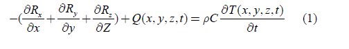
Here, R_x, R_y, and R_z denote the heat flow rates per unit area in the x, y, and z directions respectively. T (x, y, z, t) represents the present temperature, Q (x, y, z, t) is the internal heat generation rate, r stands for density, C represents specific heat, and t signifies time. This model can be further enhanced by incorporating Fourier’s law of heat conduction, which is given by:

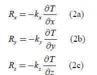
Here, k_x, k_y, and k_z represent the thermal conductivities in the x, y, and z directions respectively. Taking into account the non-linear nature of the material, the values of k_x, k_y, k_z, r, and C vary with temperature. Plugging equations (2a), (2b), and (2c) into equation (1) results in:

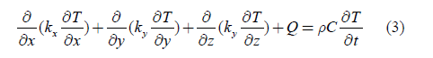
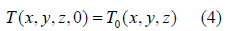
Equation (3) represents the differential equation that governs heat conduction within a solid object. The overall solution is determined by incorporating the initial and boundary conditions.

An example of an initial condition is:

boundary condition

Here, N_x, N_y, and N_z correspond to the direction cosines of the outward normal drawn to the boundary. The variables h_c and h_r represent the convection and radiation heat transfer coefficients respectively. q_s signifies the heat flux at the boundary, T₁ is the ambient temperature, and T_r stands for the temperature of the radiation heat source.

The expression for the radiation heat transfer coefficient (h_r) is

Where “s” denotes the Stefan–Boltzmann constant, “ε” is the effective emissivity, and “F” represents a configuration factor.

Mechanical model analysis

Two fundamental sets of equations concerning the mechanical model involve the equilibrium equations and the constitutive equations, which are outlined as follows:
(a) Equations of equilibrium

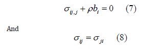
In this context, “σ_ij” represents the stress tensor, and “b_i” signifies the body force.

(b) Constitutive equations for a thermo-elasto-plastic material are expressed as follows:
The thermal elasto-plastic material model is founded on the von Mises yield criterion and the isotropic strain hardening principle. The connections between stress and strain can be formulated as follows:

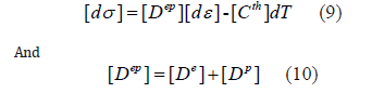
In this context, [D^e] represents the elastic stiffness matrix, [D^p] is the plastic stiffness matrix, [C^th] stands for the thermal stiffness matrix. [d^σ] indicates the stress increment, [d^ε]represents the strain increment, and “dT” signifies the temperature increment.

Analytical model for longitudinal strain

The temperature-induced deformation, denoted as εα, occurring during the longitudinal contraction, can be scientifically described as follows:

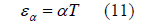
α represents the material’s coefficient of thermal expansion, indicating how much it expands or contracts with changes in temperature. T denotes the temperature measured in degrees Celsius (ºC).

The total deformation is computed by adding together the elastic, plastic, and thermal strains:

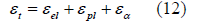
When an initial imperfection is detected prior to applying the heating load to the plates, the total deformation is influenced as follows:

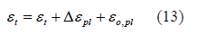
In this context, Δ_εpl represents the plastic strain that develops during the heating and cooling phases of the welding process, while ε_o,pl represents the initial imperfection observed before subjecting the plates to the heating load.

When two plates are joined by welding, the resulting distortion is primarily due to the contraction along the weld’s axis. Research conducted by Okerblom [25] has demonstrated that his method provides a highly accurate prediction for the longitudinal shrinkage caused by the temperature distribution along the weld. Okerblom’s approach is based on analytical heat-transfer theory involving moving heat sources. In his analysis, he established the distributions of thermal strain and stress around the weld. He made certain assumptions, including:
a. The coefficient of thermal expansion and the young modulus (a measure of material stiffness) are considered independent of temperature.
b. Displacements remain within the elastic range, meaning the material behaves linearly elastically.
c. Hooke’s Law, which relates stress and strain, is applicable.
d. Cross sections will be planar after deflection, meaning they won’t warp.
e. The cross-section of the material is uniform.
f. The structure is made of a single material grade.
g. The temperature distribution along the length of the welded plates is uniform and remains in a steady state.

These assumptions provide a solid foundation for Okerblom’s method, which accurately predicts the longitudinal shrinkage

caused by temperature variations during welding. Additionally, it’s assumed that the material exhibits an elasto-fully-plastic stressstrain behavior without hardening. This behavior is characterized by just two material parameters: The yield stress of the material is specified as a function of temperature within the range of 500 to 600 degrees Celsius. Within this interval, the yield stress decreases linearly, eventually reaching zero. If the temperature exceeds 600 degrees Celsius, the material does not experience any measurable stress. Several key assumptions are made in the analysis of the development of plastic strain in the welded plates during a one-pass butt-weld:
a. Heat-Induced Load: The plastic strain in the welded plates is primarily a consequence of the heat load applied during the welding process. This heat leads to thermal expansion and contraction, resulting in deformation and stress within the plates.
b. Uniaxial Stresses: The stresses experienced by the material are uniaxial, meaning they act along a single principal axis. This simplifies the analysis by assuming that the stress distribution is predominantly in one direction.
c. Quasi-Stationary Heat Load: The heat load applied to the plates during welding is considered quasi-stationary. This suggests that the thermal conditions remain relatively constant during the welding process, allowing for simplified modeling.
d. Weld Location: The weld is positioned at the middle of the two welded plates in the Z-direction. This placement is a critical factor in determining the distribution of stress and strain within the plates and simplifies the analysis by focusing on a specific location.

These assumptions help streamline the analysis of the plastic strain development in the welded plates, making it more manageable and tractable for practical applications. The thermal load can be approximated using the information provided in Figure 1c. To analyze the thermal strain, the distribution of strain in the net section l-l is considered. This section is situated in the widest part of the area where the temperature reaches 600°C. The analysis of thermal strain is conducted using the approach outlined in Okerblom [25] and Nikolaev et al. [32]. This approach likely involves applying principles and equations from these references to estimate how the material undergoes deformation and strain due to the specified thermal conditions.

In this analysis, it’s assumed that the initial plastic strain, denoted as ε_o,pl, is equal to 0. The strain induced by the temperature change, ε_α, is given by αT, where α represents the coefficient of thermal expansion, and T represents the temperature change.

The resulting strain, which is located on the straight-line l-l, is calculated as follows:

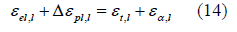
When a strip of unit width is cut from the welded plates, the strain developed by the temperature in the Z-direction is denoted as ε_α,l , and it’s calculated as ε_α,1 = -αT. This strain is shown as a bold curve in Figure 1a with a negative sign to indicate shortening or contraction. Since the strip is a part of the welded plate, the strain develops consistently and uniformly throughout the entire breadth, which is 2b in the welded plates. Figure 1b illustrates the strain development, with negative sign indicating shortening and positive sign indicating elongation strain as the temperature changes. This behavior is consistent along the entire width of the welded plates. In this context, the plastic strain is represented by crosshatching, while the elastic strain is depicted with line hatching. The position of the strain level marked as m-m′ is determined by the balance of stresses within the section l-l. It is assumed that residual stresses are proportional to the elastic strain, which can be expressed as σ=Eε_el. Based on this assumption, equilibrium can be established by considering the elastic strain resulting from the balance in residual stresses. Above the straight-line l-l, the total strain is denoted as ε_t, while below this line, the potential elastic strain is ε_el=ε_v= σ_v/E. The magnitude of ε_el is constrained by the straight-line a-c. It’s important to note that the yield stress varies linearly with temperature in the range of 500 to 600ºC. As a result, the elastic strain decreases close to zero and remains at this level at temperatures greater than 600ºC. If the elastic strain satisfies the condition ∫_-b^bε_eldy =0 , then equilibrium is confirmed. This condition likely involves ensuring that the integral of elastic strain within the specified limits matches the negative integral from 0 to some point, confirming the balance of forces and stresses within the welded structure. The width of the region labeled as “b₁” exclusively represents elastic strain. In contrast, the combined widths of “b₂,” “b₃,” and “b₄” collectively cover both elasto-plastic and plastic strain. Within these regions, “b₂,” “b₃,” and “b₄,” the total area covered is indicative of the plastic strain area, denoted as “2b_pl.” This means that the sum of the widths of these three sections represents the extent of the plastic strain within the material. To determine the residual strain and stresses, it is necessary to analyze the strain that occurs during the cooling process, taking into account the strain distribution at sections 1-1 and 2-2 after the cooling process has reduced the temperature to 0ºC. In this context, the initial plastic strain is the one that was generated during the heating process in section 1-1, represented as ε_pl.0.2 = Δε_pl,1. Additionally, the thermal strain at this stage, ε_α.2, is equal to 0 due to the temperature being reduced to 0ºC. So, the situation can be summarized as follows:

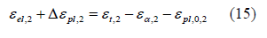
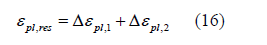
The curve represented by “kfpf′k′” characterizes the left side of Equation (15), which accounts for both elastic and the incremental plastic strain developed during the cooling process. To distinguish between the elastic and plastic strains, it’s necessary to consider the proportional limit at room temperature. This involves identifying the maximum elastic strain, denoted as ε_el,max = ε_v = σ_v/E. The crosshatched area, “fpf′,” corresponds to the plastic strain in elongation, Δεpl,2, resulting from the cooling process, while the line-hatched area represents the elastic strain. If the integral of the elastic strain within the specified limits, ∫_-b^bε_eldy =0, evaluates to zero, then the straight line is correctly positioned, confirming equilibrium. The residual plastic strain, Δε_pl, is the sum of the plastic strain that occurred during heating and the plastic strain induced by the cooling processes:

Residual stresses can be calculated by multiplying the residual strain by the modulus of elasticity (E). The area marked by “a-f Residual stresses can be calculated by multiplying the residual strain by the modulus of elasticity (E). The area marked by “a-ff′- a′” represents the thermal shrinkage impulse force, denoted as AT. This force is responsible for generating the residual stresses and the subsequent shrinkage in the welded plates.

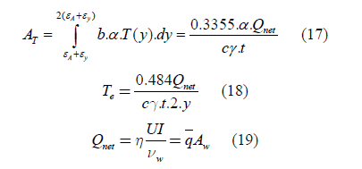
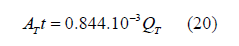
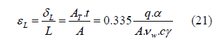
The thermal impulse (A_T) is determined by factors such as the arc voltage (U), arc current (I), welding speed (v_w), specific heat of the material (c), material density (γ), plate thickness (t), coefficient of efficiency (η), specific heat of the unit welded joint area (q, for a 1 mm² area), and the size of the welded joint area (A_w). This thermal impulse represents the heat input into the welding process and is calculated based on these parameters, with the specific formula varying depending on the welding method, materials, and welding conditions being used.

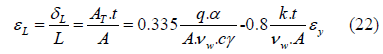
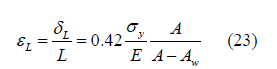
The fundamental formula for longitudinal strain as proposed by Okerblom[25] is determined as follows:

The Okerblom [25] model operates on the assumption that the welding material is deposited uniformly over the entire length of the weld at the same time. This model is particularly applicable when dealing with fast-moving heat sources or relatively short welds. In a review of theoretical prediction models for distortion, which was compiled from a comprehensive study by Verhaeghe [33], several models are discussed. One of these models is attributed to Wells [34]. Wells [34] expanded upon the Okerblom [25] model and enhanced predictions for longitudinal strain by incorporating the impact of temperature distribution that occurs perpendicular to the weld.

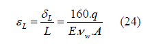
The Pflug model from 1956 operates on a similar rationale as the Okerblom model. However, in the Pflug model [35], the area undergoing plastic deformation, as originally defined by Okerblom [25], is substituted with a ratio related to the weld area. This model shares some of the same limitations as the Okerblom model.

White et al. [26] introduced a model for longitudinal shrinkage that stands out by considering the effects of process efficiency, a factor that had not been taken into account in previous models. This addition made their model more comprehensive and improved its accuracy in predicting longitudinal shrinkage during welding processes.

Validation of numerical modeling

For validating the results of numerical models, experimental test results conducted by Hashemzadeh were utilized. Hashemzadeh joined two 4-mm thick plates using a welding process at a speed of 6.25 mm/s. Figure 2 displays the geometric specifications and boundary conditions of the laboratory sample. The mechanical- thermal properties of ASTM A36 steel are outlined in Table 1. To perform numerical simulations, a sequential analysis method was employed. Initially, dynamic thermal analysis was conducted, followed by transforming the thermal elements into structural elements, with the results of the thermal analysis serving as loads for the structural analysis. For the thermal analysis, the 3D Solid70 element was used, and for the structural analysis, the 3D Solid185 element was employed. To simulate the nonlinear behavior of steel, considering both yield and isotropic hardening, Von Mises yield criteria [36] were taken into account. The convective coefficient, plate temperature, and ambient temperature were all assumed to be 25 °C. To simulate the welding process in the thermal analysis, birth and death elements were used. The welding was performed as a single-pass weld at a speed of 6.25 mm/s with a temperature of 1500°C.

Table:Temperature-dependent material properties, ASTM A36.

In Figure 3a & 3b, a representation of thermal analysis and longitudinal distortion in the numerical model is depicted. Figure 3c shows a temperature chart at a distance of 10 mm from the weld line in both the numerical and laboratory models, demonstrating that the thermal simulation results exhibit a good match with experimental results. In Figure 3d, the deformation values at the end of the welding process are illustrated for the numerical and laboratory models, indicating that the numerical results have an acceptable level of accuracy. Figure 3d displays the distribution of residual stresses across the width of the plate. Neglecting residual stresses in calculations can lead to premature component failures.

Results

In this section, an examination was conducted on the longitudinal distortion resulting from welding in steel plates. A plate with dimensions of 500 x 300 millimeters and mechanical-thermal properties as specified in Table 1 was considered. To account for the effect of thickness and welding speed, plate thickness ranged from 1mm to 7mm with a 1mm increment, welding speeds varied from 1mm/s to 3 mm/s with a 0.25 mm/s increment, and from 3 mm/s to 10 mm/s with a 0.50 mm/s increment. In Figure 4, the impact of welding speed on the heat distribution at a distance of 10 mm from the weld line is illustrated. As welding speed increases, the maximum temperature decreases because less heat flux is introduced to each part, resulting in a reduction in the maximum temperature. Considering that the heat distribution in welding on plates depends on thickness and welding speed, Figure 5 illustrates the maximum temperature at a distance of 10 mm from the weld line based on thickness and welding speed. As evident from the graph, reducing the plate thickness leads to a decrease in the maximum temperature, although this reduction is not significantly pronounced. Additionally, as welding speed increases, the maximum temperature decreases. In contrast to the effect of thickness, the welding speed parameter has a substantial impact on the maximum temperature.

Increasing welding speed can reduce changes in the volume of metal, thereby affecting the resulting strains. It’s important to note that in reality, extremely low or extremely high welding speeds are not feasible. Very low speeds can result in inadequate fusion of the welding filler material, while very high speeds can prevent the filler material from fully filling the weld seam. In the next section, we will examine the impact of welding speed on longitudinal distortion resulting from welding. Imagine a welded joint, specifically the part where the weld was made and the area just behind it. This region gets squeezed because it’s surrounded by the stiff, cold material of the base metal. This squeezing is balanced by pulling forces on both sides of the squeezed area along the rest of the metal. As the welding torch moves away and this squeezed region cools down, the stress situation changes. Now, instead of being squeezed, the region experiences pulling forces, while the rest of the metal is under compression. If the metal in the plate can’t effectively withstand these pulling forces, it will shrink lengthwise. In practical terms, we usually estimate that for every 3 meters of weld, fillet welds typically shrink by about 0.8mm, and butt welds shrink by about 3mm. Over time, scientists and experts have tried to create equations to predict this type of distortion more accurately, but these equations haven’t proven to be very precise. In the Figure 6, the results of finite element analysis of numerical models with varying thickness and welding speed are presented. It is evident that an increase in welding speed leads to a reduction in longitudinal distortions.

Based on numerical simulations and prior studies, it is clear that as welding speed goes up, the longitudinal distortion tends to decrease. This happens because when the welding speed is higher, the input energy required for welding decreases. This net input energy is determined by factors like arc voltage (U), arc current (I), welding speed (vw), and the efficiency coefficient (η). Through sensitivity analysis, it was determined that the tendon force parameter is inversely related to the welding speed following an exponential distribution. Therefore, the longitudinal distortion is calculated according to the equation (27).

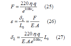
The coefficient of determination (R²) value of 0.989 indicates a strong correlation between the finite element models and the equation (27). As observed in Figure 7, the equation (27) exhibits a good fit with the reference experimental results [37]. The comparison in Table 2 between the results of the equation (27) and the results of past equations and experimental [37] data shows that the provided equation aligns well with the experimental results. Based on Table 2, the equations proposed by researchers in the past significantly differ from the experimental results and underestimate the longitudinal distortions. However, the equation (27), derived from finite element analysis results, exhibits an acceptable level of accuracy with a 10% error compared to the experimental data.

Table 2:Comparison of Longitudinal Distortion Prediction to Experimental Data and Previously Calculated Longitudinal Distortions.

Conclusion

In this study, longitudinal distortion was investigated considering the variables of welding speed and steel plate thickness. In general, as each of these two variables increases, the magnitude of longitudinal distortion decreases. The maximum longitudinal distortion occurs at the weld line and decreases as you move away from the weld line. To examine longitudinal distortion, first, the numerical model results were validated against experimental results. Then, plate thickness ranging from 1 millimeter to 7 millimeters and welding speeds from 1 millimeter to 10 millimeters per second were considered as variables. According to the finite element analysis results, a relationship with an R2=0.989 was proposed. This provided equation demonstrated a good match with the experimental results. The average error of the proposed equation with respect to the experimental results was 11.5%, while previous equations had errors as high as 92%. It appears that considering all types of distortions would lead to better predictions.

References

1. Saha J, Barman B, Chouhan PJC (2020) Lockdown for COVID-19 and its impact on community mobility in India: An analysis of the COVID-19 Community Mobility Reports 116: 105160.
2. Li A, Zhao P, Haitao H, Mansourian A, Axhausen KWJC (2021) How did micro-mobility change in response to COVID-19 pandemic? A case study based on spatial- temporal-semantic analytics 90: 101703.
3. Tuli FM, Nithila AN, Mitra SJTRIP (2023) Uncovering the spatio-temporal impact of the COVID-19 pandemic on shared e-scooter usage: A spatial panel model 20: 100843.
4. De Vos JJTrip (2020) The effect of COVID-19 and subsequent social distancing on travel behavior 5: 100121.
5. Menon N, Keita Y, Bertini RL (2020) Impact of COVID-19 on travel behavior and shared mobility systems.
6. Lekić Glavan O, Nikolić N, Folić B, Vitošević B, Mitrović A, et al. (2022) COVID-19 and City Space: Impact and Perspectives 14(3): 1885.
7. Almannaa MH, Ashqar HI, Elhenawy M, Masoud M, Rakotonirainy A, et al. (2021) A comparative analysis of e-scooter and e-bike usage patterns: Findings from the City of Austin, TX. International Journal of Sustainable Transportation 15(7): 571-579.
8. McKenzie G (2019) Shared micro-mobility patterns as measures of city similarity: Position paper. Proceedings of the 1st ACM SIGSPATIAL International Workshop on Computing with Multifaceted Movement Data.
9. Padmanabhan V, Penmetsa P, Li X, Dhondia F, Dhondia S, et al. (2021) COVID-19 effects on shared-biking in New York, Boston, and Chicago 9: 100282.
10. Yang H, Huo J, Bao Y, Li X, Yang L, et al. (2021) Impact of e-scooter sharing on bike sharing in Chicago 154: 23-36.
11. Yan X, Yang W, Zhang X, Xu Y, Bejleri I, et al. (2021) A spatiotemporal analysis of e-scooters’ relationships with transit and station-based bikeshare 101: 103088.
12. Tuli FM, Mitra S, (2021) Factors influencing the usage of shared E- scooters in Chicago 154: 164-85.
13. Bai S, Jiao J, Chen Y, Guo JJ (2021) The relationship between E-scooter travels and daily leisure activities in Austin, Texas 95: 102844.
14. Noland RBJF (2019) Trip patterns and revenue of shared e-scooters in Louisville, Kentucky.
15. Fistola R, Gallo M, La Rocca RAJ (2022) Micro-mobility in the “Virucity”. The Effectiveness of E-scooter Sharing 60: 464-471.
16. Teixeira JF, Lopes MJ (2020) The link between bike sharing and subway use during the COVID-19 pandemic: The case-study of New York's Citi Bike 6: 100166.
17. Brown A, Williams RJTRR (2023) Equity implications of ride-hail travel during COVID-19 in California. 2677(4): 1-14.
18. Wielechowski M, Czech K, Grzęda ŁJE (2020) Decline in Mobility: Public Transport in Poland in the time of the COVID-19 Pandemic. 8(4): 78.
19. Engle S, Stromme J, Zhou AJAa (2020) Staying at home: mobility effects of covid-19.
20. Molloy J, Schatzmann T, Schoeman B, Tchervenkov C, Hintermann B, et al. (2021) Observed impacts of the Covid-19 first wave on travel behaviour in Switzerland based on a large GPS panel. 104: 43-51.
21. Beria P, Lunkar VJSC (2021) Presence and mobility of the population during the first wave of Covid-19 outbreak and lockdown in Italy 65: 102616.
22. Galeazzi A, Cinelli M, Bonaccorsi G, Pierri F, Schmidt AL, et al. (2021) Human mobility in response to COVID-19 in France, Italy and UK 11(1): 13141.
23. https://www.chicago.gov/content/dam/city/depts/cdot/Misc/EScooters/2021/2020%20Chicag o%20E-scooter%20Evaluation%20-%20Final.pdf
24. https://data.cityofchicago.org/Transportation/E-Scooter-Trips-Census-Tract-Summary- 2020/3srm-twg4 E-st-Cts-CoCDP