 Research Article
Improving the Predictive Power of Marine Species Distribution Models by Incorporation of Modelled Prey Data
Lars O Mortensen1*, Jonas B Mortensen1, Ingrid Ellingsen2, Mathias Singsaas Frøseth1 and Henrik Skov1
1DHI A/S, Denmark
2SINTEF Ocean, Norway
Lars O Mortensen, DHI, Agern Allé 5, DK-2970 Hørsholm, Denmark.
Received Date: December 10, 2021; Published Date: February 01, 2022
Abstract
Species distribution modelling (SDM) often relies on hydrodynamic processes as proxy for prey items, when estimating animal distributions at sea. This is due to the fragmented nature of prey data available, which makes the data ill-suited for SDM. However, the incorporation of prey data remains an unresolved potential with the outcome of studies so far being ambiguous. To assess the potential effect of including modelled data on prey density in marine species distribution models developed solely on dynamic variables we used a dynamic modelling framework MARAMBS for prediction of the fine-scale densities and movements of seabirds in the Barents Sea. We tested the effect of incorporating synoptic modelled data on calanoid zooplankton from the SINTEF SINMOD model into this SDM framework for the planktivorous Little Auk (Alle alle). Copepods constitute the main prey of the little auk which breeds in the northern parts of the Barents Sea and makes seasonal migrations out of the region to/from wintering grounds further south off the Norwegian coast.
The approach consisted of a three-step process. Hydrodynamic variables were derived from a 3d oceanographic model developed, while prey information was derived from the SINMOD model. The derived information was coupled with observation data on the Little Auk in a generalized additive model (GAM) to predict the spatio-temporal distribution of the auk. Predictions were made in three-hour time steps, yielding a spatial timeseries on species density across the study area. GAMs were conducted with and without prey information to estimate model improvements. Furthermore, predicted species densities from GAMs were converted into spatio-temporal habitat suitability index (HIS), which served as a prey information for an Agent Based Model (ABM), simulating the migratory patterns of the Little Auk in the Barents Sea. Simulations were subsequently performed with initial HSI (no prey), prey HSI (HSI with prey information) and a simulation with baseline HSI and prey information separate but parallel. Simulations were validated against observations using Goodman and Kruskal’s gamma.
Results showed that both GAM’s and ABM performed significantly better with the inclusion of prey information. The most significant improvement was seen when incorporating prey HSI, where the prey information was included in the GAM and used to drive predicted movements of Little Auks by the GAM. Thus, the results show that the addition of a prey item as a predictor variable is highly likely to improve SDM predictions in comparison with existing models driven alone by oceanographic variables. At the same time, replacing oceanographic predictors with the prey information resulted in poorer model performance indicating inefficient detection of prey patches by the seabirds.
Introduction
It has become standard in marine species distribution modelling (SDM) studies to use oceanographic proxies for prey, as hydrodynamic processes often are the main drivers of marine animal feeding habitats [1-3]. Yet, oceanographic proxies are typically used because of the fragmented nature of available surveyed prey data which makes them inappropriate for use in SDM. However, by relying entirely on the use of oceanographic proxies may limit the transferability of SDM as prey may constitute an important aspect of the realized niche [4] and could limit the ability to use the SDM for forecasting distributions because the relationships between the proxies and prey distribution or density may change in a changing climate [5-7]. It is also worth stressing that the predictive power of hydrodynamic predictor variables obtained from limited in situ and modelled oceanographic data may not represent the fine-scale processes important to foraging, such as processes that aggregate prey into concentrations sufficient to trigger predator feeding activity [8, 9].
The enhancement of marine habitat and species distribution models by incorporation of prey data remains an unresolved potential, as results of studies testing the potential have been ambiguous. Torres et al. [10] showed that incorporating prey data as an explanatory variable into fine-scale models of habitat selection of bottlenose dolphins within a heterogeneous coastal environment did not improve predictive power. Conversely, several studies have demonstrated that the use of prey data improved the performance of ecological models for fishes [11-13], sharks [14], birds [15] and cetaceans [16,17]. However, recently [18] made formal assessments of the value of using modelled zooplankton prey versus physical variables for predicting bowhead whale (Balaena mysticetus) habitat use. They concluded that the best model included bathymetry and modelled hydrodynamic and prey variables. Inclusion of dynamic variables in SDMs produced predictions that reflected temporal dynamics evident from the survey data. Due to the stability of bowhead distribution bathymetry was the most influential variable in models that included that variable.
In order to assess the potential effect of including modelled data on prey density in species distribution models developed solely on dynamic variables we used a dynamic modelling framework MARAMBS for prediction of the fine-scale densities and movements of seabirds in the Barents Sea [19]. We tested the effect of incorporating synoptic modelled data on calanoid zooplankton from the SINTEF SINMOD model [20,21] into this SDM framework for the planktivorous Little Auk (Alle alle). Copepods constitute the main prey of the little auk which breeds in the northern parts of the Barents Sea and makes seasonal migrations out of the region to/ from wintering grounds further south off the Norwegian coast [22].
Method
Study area and species
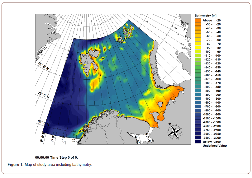
The models used for species distribution modelling in this research was developed in the project Marine Animal Ranging Assessment Model Barents Sea [19], which focused on the species distribution of the Little Auk (Alle alle) in the Barents Sea, which subsequently also was the study area used in the current research (Figure 1).
Modelling framework
We used the MARAMBS model framework which incorporates fully integrated 3-D hydrodynamic models, dynamic habitat suitability models and agent-based models [23]. For detailed information on hydrodynamic, static, and observational data, please see MARAMBS report [19].
Observational data
Observational data on the Little Auk was derived from the Norwegian Ecosystem Surveys in the Barents Sea (Prozorkevich & Sunnanå, 2017), which covered surveys from the period 2004 to 2016.
Hydrodynamic model data
The study included data on hydrodynamic conditions in the study area over the period 2004-2016, which was derived from using DHI’s 3-dimensional flexible mesh model package MIKE 3 FM https://www.mikepoweredbydhi.com/products/mike-3,which includes both meteorological, tidal and oceanographic effects. Modelled oceanographic data included sea surface temperature, salinity and ice cover, along with a measure of distance to the Polar Front.
SINMOD configuration and plankton modelling
Zooplankton data have been produced by SINMOD, a fully coupled hydrodynamic-ice-chemical-biological model system. The hydrodynamic component of the model system, which is responsible for calculating the basic physical properties of the ocean like velocity, water temperature and pressure, is based on the so-called primitive Navier-Stokes equations. The model is forced by atmospheric data: wind, heat exchange, tides and freshwater runoff from land [20]. The ice model is like that of Hibler [24]. The ice momentum equation is solved together with an equation for the ice internal stress, using the elastic-viscous-plastic (EVP) dynamical model of [25].
The ecosystem model component of SINMOD is primarily nitrogen (NO3, NH4) and silicate based. It is formulated in a Eulerian framework. The state variables describe basic components of the microbial loop food web (bacteria, heterotrophic nanoflagellates, diatoms and autotrophic flagellates, ciliates) as well as two key mesozooplankters: the Atlantic Calanus finmarchicus and the arctic C. glacialis. SINMOD operates with 2 boxes for detritus, one fast and one slow sinking. An explicit bacterial component is included into SINMOD, which also includes DOC dynamics to assess losses resulting of algal leakage and zooplankton sloppy feeding (leading to breaking of algae cells under conditions with high food concentration).
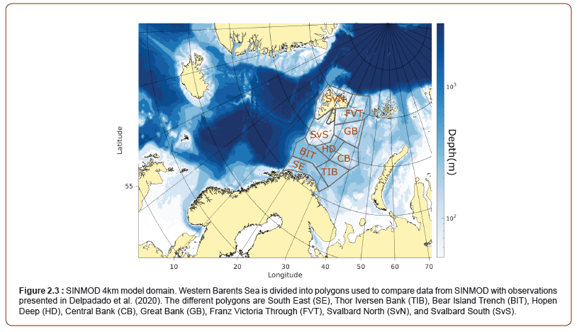
Growth of phytoplankton is simulated as a function of available light and nutrients [21]. Light penetration beneath ice is calculated following a model by Pegau et al. [26]. In ice covered waters, primary production in each grid cell is calculated as the sum of production under ice covered part and the open water part of the grid cell. The model domain of SINMOD with 4 km horizontal resolution is shown in Figure 2. The model is nested to a regional model setup with 20 km horizontal resolution. More information about model setup and forcing can be found in Wassman et al. 2021 and [27].
Output from SINMOD have been saved daily for use in the MARAMBS framework from simulations with both 20 km and 4 km spatial resolution.
Habitat suitability modelling/Prediction using generalized additive modelling
The benefits of using information on prey distribution was initially tested using a generalized additive modelling approach for assessing the species distribution of the Little Auk in a Hurdle setup. Initially, the Hurdle model for the species distribution was made using dynamic hydrodynamic conditions as explanatory variables. The initial SDM was based on the SDM used previously in the MARAMBS project [19]. This model included the environmental variables listed in Table 1, as explanatory variables and species densities in each transect segment as dependent variable.
Table 1: Environmental variables included in modelling. The depth at which each oceanographic variable was extracted from the hydrodynamic model is indicated.

The model was fitted as a generalized additive mixed model (GAMMs) using the “mgcv” R package (Wood, 2006). The presenceabsence component of the hurdle model was fitted with a binomial distribution, while the positive component was fitted a quasipoisson distribution. Each explanatory variable was fitted as a smooth term (k = 3) and the correlation structure was fitted using the time of observation. Potential residual autocorrelation was analyzed using the gam.check function in “mgcv”.
Next, the SDM was expanded using the modelled distribution of Calanus derived from the SINMOD model. As the SINMOD models data was available in both 4 km and 20 km resolution, a first set of models were developed to estimate which resolution added the most, if any, explanatory power to species distribution model (SDM). This was completed on a single year (2016) of data, to speed up the modelling process. Secondly, the most appropriate resolution was then extracted to a full 9-year data series and a new SDM was developed, based on the existing model.
Subsequently, predicted densities were mapped based on both the initial and the extended model. The performance of each model was then evaluated by correlating the predicted densities to the observed densities using Goodman and Kruskal’s gamma. Comparisons were conducted on different spatial scales to estimate optimal scale for comparisons.
Agent based modelling
To expand the assessment of the potential effect of prey inclusion in SDM, we applied the prey information to an Agent Based Model (ABM) designed to simulate the migration patterns of the Little Auk in the Barents Sea. The ABM called CBIRD (for Seabird) was originally designed and implemented in the project MARAMBS, to simulate the dynamic species distribution of multiple seabird species in the Barents Sea on a fine spatiotemporal scale [19]. The backbone of CBIRD is a dynamic bioenergetic module, which has profound impacts on a seabird’s decision to move on both short and long spatiotemporal scales [19] (DHI, 2016). The ability to find and capture prey for a seabird is therefore essential to the performance of the bioenergetic module, and consequently movement and dispersal of CBIRD agents in the model [19]. A key assumption in the original implementation of CBIRD is that the utilized Habitat Suitability Index (HSI) does not only represent areas that birds actively seek and intrinsically prefer to stay in, but also that the value of HSI was directly linked to the agent’s probability of finding and capturing prey items. However, this assumption has historically been a topic of much debate seeing as HSI originally did not include prey items as a predictor variable.
Prey information was incorporated into CBIRD by three overall approaches on two different spatial scales. First, normalized spatiotemporal prey densities (0-1) of Calanus were used to replace the original habitat suitability index (HSI) for little auk, to investigate if prey as a single variable can replace the composite HSI variable. Secondly, normalized spatiotemporal prey densities were added as a new input variable in the CBIRD model alongside the original HSI input variable. Thirdly, as a new updated Habitat Suitability Index map where the HSI was derived from the previous SDM using GAM analysis, where predictions were normalized to an index from 0 – 1 indicating areas of high and low habitat suitability.
The following treatments were established to determine the best method for including dynamic Calanus densities within the existing architecture of the CBIRD model (Table 2).
Table 2: Table of treatments done to the existing calibration of the CBIRD model for Little Auk. Note that Treatment ID’s in the far-right column will be used in the main text as reference to the specific treatments in following sections.

The treatments, P04 and P20, were made to investigate the hypothesis that the dynamic density-distribution of Calanus is sufficient to accurately predict the distribution of Little Auk in time and space, or in other words; is HSI even required when Calanus densities are available as direct model input. Both the 4km and 20km Calanus datasets were used to understand which resolution is best suited for the underlying triangular flexible mesh resolution of the CBIRD model. No other parameter in the model was changed for these treatments.
The treatments, HP04 and HP20, were established to clearly distinguish Calanus density-distributions from the Habitat Suitability Index, by including Calanus as a separate input variable next to HSI. The treatment thus required a change to the CBIRD formulation of how an agent detects Calanus as well as its probability of catching Calanus. The original base formulation for probability of Calanus detection, P_d, in CBIRD is given in Eq. 1 and adapted from Esposito et al. [28].
Pd =1-e-γ*Ap Equation 1
Where γ is a user-defined constant denoting the search efficiency of the agent and A_p is the relative Calanus abundance. The relative abundance has up until now has been represented by the Habitat Suitability Index, but for treatments HP04 and HP20 the variable A_p is instead linked to the normalized Calanus densities of 4km and 20km resolution. Once Calanus has been detected in the given timestep, the value of, P_d, is further used in the model to calculate how many of the foraging dives the agent will try to make in the given timestep duration that are successful. This is done by sampling from a binomial distribution with the probability of success being denoted by P_d and with n trials, where n is the model calculated number of dives the bird will attempt. The number of dives an agent will attempt depends on the size of the model timestep and its current satiation level, e.g. a hungry CBIRD agent will try to make more dives than an agent that is almost full.
Calanus ingestion in turn directly affects the satiation level (SL, range: 0-1) of the agent, which is a key parameter in CBIRD. The satiation level determines a number of important movement decisions in CBIRD, which can be summarized as follows:
• An agent will go into REST mode when Satiation Level is above a user-defined threshold. When in REST mode, the agent has no active movement and is dispersed via drifting relative to currents and winds only.
• An agent will be less likely to go into FLIGHT mode on a full stomach, but rather wait until consumed Calanus has been digested.
• When an agent achieves a Satiation level above 0.5, it will store the location in its memory as the place it will return to if future habitat does not produce the same foraging success.
No direct directional response to the new Calanus density was implemented, meaning that an agent cannot detect a gradient in the Calanus abundance beyond its sensory capacity and decide to follow it towards a higher abundance. An agent can however still detect gradients in the Habitat Suitability Index and move towards higher HSI. This logic follows the hierarchical patch dynamics paradigm [29] which implies that seabirds have an intrinsic understanding of their environment and select habitats which are beneficial to their fitness but may not necessarily be able to fully utilize the highest available Calanus densities.
The final treatment of NHSI, the new and updated Habitat Suitability Index, which includes Calanus densities as a predictor (this study) was used instead of the original HSI input. This approach is, relative to the original formulation and architecture of the CBIRD model, seen as the most fitting, seeing as there’s always been an underlying assumption in the design of the CBIRD model that HSI was also a proxy for where to find prey.
To assess the effect of each Treatment on the existing level of calibration, the Gamma Rank correlation coefficient for August and September observations was calculated on 10 different spatial scales for each Treatment and compared to the most recent calibration (without Calanus) for Little Auk in the year of 2016. To establish whether the change in calibration was considering statistically significant, a Student’s Paired T-test was made to compare the correlation coefficients between baseline and treatment.
For further analysis relative to investigate changes in seasonal distribution and migration patterns, mean densities were calculated for the Autumn (Aug-Oct) and Winter (Nov-Dec) seasons, and compared relative to the calculated population loss due to migration.
Results
Evaluation of SINMOD results
Model output from SINMOD have previously been validated by Lee et al. [30] and Vernet, et al. [27], but last validation of zooplankton distribution was done by Ellingsen et al. [31] . In this study we have used observations reported on Dalpadado et al. [32] and compared onset of spring bloom start day and zooplankton biomass (Table 2).
The estimated start date of spring bloom from SINMOD 4 km resolution and satellite data are overall in good agreement, with some exceptions. The model predicts a later start of the spring bloom in TIB (Figure 2.3) both in 2013 and 2016. The satellite data show a very late bloom start for the FVT (Figure 2.3) polygon in 2013 that is not captured by the model. In 2016, bloom start day estimates are very similar in this region. T In 2016, the satellite estimate gives also a later start than SINMOD in SvN (Figure 2.3) in 2016.
Mesozooplankton distributions
Observations of mesozooplankton biomass within the different polygons (Figure 2.3) are found in Dalpadado et al. [32] and compared to model estimates in Table 2. The spatial and temporal variability are higher in the observational data compared to the model data. Since the model results used estimates are averaged over the month (August), while the observations represent the biomass on the sample day, and less variability in the model estimates should thus be expected. Distributions of mesozooplankton biomass in 2013 and 2016 are shown in Figure 2.10. Simulated biomass of mesozooplankton is lower over the Svalbard Bank, the Central Bank and the Great Bank than in the deeper regions and this pattern is also found in measurements [32]. Observation data show generally higher biomass in 2016 compared to the 2013 data. The model estimates are more similar for the two years. The maximum simulated biomass in August, however, is generally higher in 2016 than in 2013 (Figure 2.10).
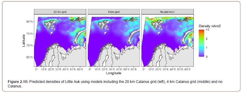
Table 3: Results from SINMOD (4km model) and measurements from Dalapado et al. [32], data from supplementary document) for the different polygons shown in Figure 2. SINMOD provide biomass estimates in gC and a conversion factor of 0.525 has been used to convert to g dry weight [36].

Comparing Calanus model resolution
The baseline SDM and models with two Calanus resolutions were fitted for the 2016 data. Generally, the three models displayed the same R2 value (Table 3). The model with no Calanus data included exhibited the lowest degree of variance explanation, followed by the 4km resolution and then the 20 km resolution.
Table 4: Overview of model results from three habitat models, with either no Calanus data, Calanus in 4 km grid resolution or 20 km grid resolution.
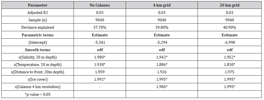
Comparing the three models using an Analysis of Variance (ANOVA), both models using Calanus showed a significant lower degree of residual deviance than the model with no Calanus data. Additionally, the model using the 20 km grid resolution also had a lower degree of residual deviance than the model using the 4 km grid resolution, however the difference was not significant (p > 0.05).
Despite the lack of significant difference in residual deviance, predictions of density from each model varied greatly (Figure 2). The large aggregations predicted in the no Calanus model in the northern part of the study area were not present in both models which applied Calanus data. In the no Calanus model, this was seemingly an effect from the Ice predictor, which were less pronounced in the Calanus models. Between the Calanus models, there were a less effect on the distribution predicted, although the densities were predicted to be larger in the 20 km grid resolution, than in the 4 km resolution. Thus, based on the predictions above and the summary statistics on the models, the addition of Calanus did improve the habitat models. Additionally, while the difference between the 20 km grid resolution and the 4 km grid resolution was not very large, there was an indication of the 20 km grid resolution was better suited for the models than the 4 km grid resolution.
Dynamic Habitat Predictions
The 20 km grid resolution plankton data was selected as adding most information to the 2016 model data. Subsequently, this data was extracted for the years 2004-2014 and was used to update the original MARAMBS model for Little Auk, which covered the same time span. Results from the updated model and original model can be seen in Table 4. As expected, the addition of the plankton yielded a slight increase in model fit. The updated model was then used to predict hourly densities across the study area, using the dynamic hydrodynamic and Calanus predictors. This yielded a spatial time series of densities, which were subsequently transformed into a habitat suitability index.
Agent based modelling
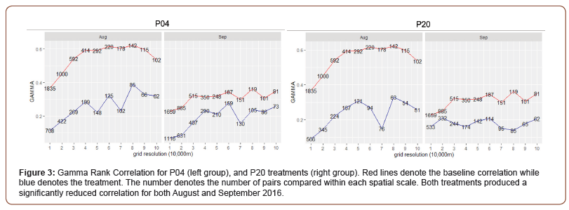
The P04 and P20 treatments both resulted in a significant reduction (p < 0.01) in correlation coefficient between the existing baseline calibration and the two treatments (Figure 3). The drop in correlation was most profound in the month of August, but September was consistently below original values as well.
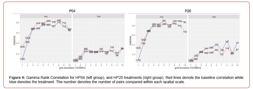
The treatments, HP04 and HP20 proved to be performing better (Figure 4) than the P04 and P20-treatments, however HP04 still resulted in a significant drop in correlation between baseline and treatment (p < 0.01) during August and across all scales. For September, HP04 performed slightly better on small spatial scales, however the differences were not tested to be significant (p > 0.05). For HP20 there was a similar drop in correlation on small spatial scales (10-20km), but generally improved correlation on larger spatial scales. However, the differences for August were tested to be insignificant (p > 0.05). For September there was an almost consistent improvement in the correlation, which also tested to be statistically significant (p < 0.01). The results for HP20 are consistent with the earlier findings during the GAM revision, which also had the biggest increase in predictive power with the 20km resolution dataset.
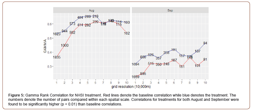
The final treatment (NHSI) using the new and updated HSI revealed a statistically significant (p < 0.01) high increase in the Gamma Rank correlation across nearly all spatial scales for August and September 2016 (Figure 5). Most noteworthy is the large increase in correlation for small spatial scales (10-20km) relative to previous calibrations.
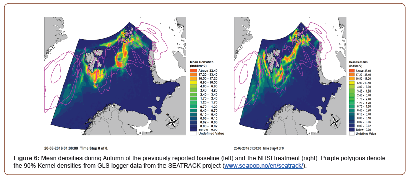
As the NHSI treatment produced by far the largest increase in correlation, this treatment was selected for further inspection and analysis relative to initial model. Mean densities during the autumn (Aug-Oct) and winter (Nov-Dec) were calculated and compared to the results previously reported for Little Auk during the MARAMBS projects [19].
As seen in Figure 6, the NHSI treatment have a rather profound effect on the predicted distribution of Little Auks. The population from West Spitsbergen have moved further west, whereas the Bjørnøya population is seeking further northeast, rather than due north as they did in the initial predictions. The majority of agents from Franz Joseph Island has become ‘faster’ and more directional in their westward migration. Overall, the distribution in the fall has been become less aggregated than previously predicted, with many smaller high-density patches of Little Auk, which upon visual comparison with the 90% GLS Logger kernel densities from the SEATRACk project (www.seapop.no/en/seatrack/) seem to have a better fit.
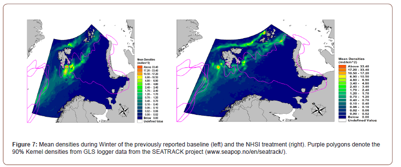
By winter (Figure 7) a relatively larger part of population originating from the colonies in West Spitsbergen and Bjørnøya has migrated outside of the domain, which can be seen by the lower densities in these areas. The migration of colonies in the most northern Franz Joseph islands have however slowed by the increased densities relative to the initial baseline prediction. The changes in autumn and winter distribution patterns can also readily be seen in the ‘loss’ of the simulated agent population due to the short- and long-term migration of agents during the simulation (Figure 8).
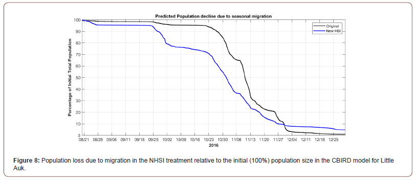
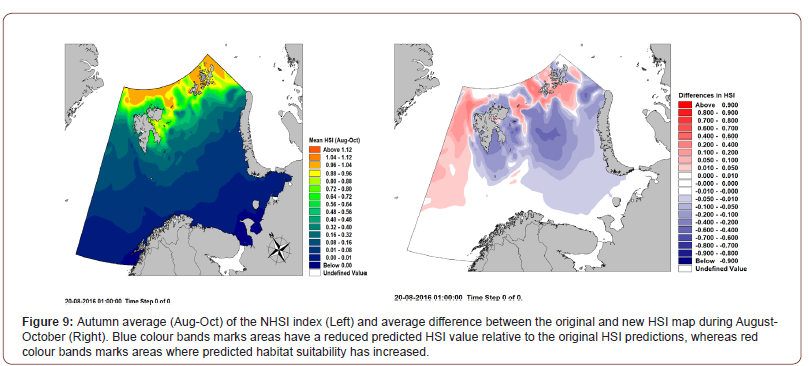
As it is apparent from Figure 8, the new Habitat suitability has resulted in an earlier onset and steeper decrease in population from end September until end November. The reason for this is likely due to the spatial shift in HSI, which is now relatively higher at the western boundary of the Barents Sea and is thus allowing westward migration from the Barents Sea through areas of enhanced HSI. At the same time, the new HSI limits high latitudinal migration of some of the colonies from Franz Joseph Islands. This can be explained by the increase of HSI in the vicinity of Franz Joseph Islands (Figure 9), which in turn results in the agents not migrating very far from Franz Joseph during their flightless migration period.
Discussion
Both the habitat model and the agent-based model in the MARAMBS SDM framework benefited from the inclusion of modelled Calanus prey as a predictor variable. However, the effect was not the same for both models and varied with usage.
Performance of habitat suitability model
For the habitat model, the addition of information on Calanus availability increased the model fit slightly, with a tendency for a coarser grid (20 km grid) having a better fit. This is likely due to a ‘loose’ association between schooling zooplankton and Little Auk in offshore areas and it corroborates the general view of inefficient detection of prey by seabirds feeding on patchily distributed prey [33, 34]. Thus, the Calanus distribution served to a higher degree as an indicator of areas of high productivity, in concert with the hydrodynamic variables, rather than as an indicator of the location of patches of Calanus. Furthermore, transforming the models into dynamic predictions, the inclusion of a prey item greatly increased the correlation between model predictions and survey observations. Thus, while it is assumed that the hydrodynamic variables in the habitat models are proxies for areas with good food availability, adding an actual food source to the model seems to underpin the models and improve the spatiotemporal patterns predicted by the models.
In contrast, the application of the Calanus distribution into the agent-based model showed a varying effect, depending on the usage of the food availability. Applying only the food source resulted in poorer model performance than using only hydrodynamics, stressing the indications of inefficient detection of prey patches by seabirds. This was supported by the inclusion of the habitat suitability maps in the simulations, where both HSI and Calanus distribution worked in concert. This resulted in model fits equivalent to previous models, indicating that the HSI was the main driver of the distribution. However, incorporating the Calanus distribution into the HSI through the habitat suitability modelling resulted in improved model predictions, disproportionate to the level of improvement to the habitat model fit. This result indicated that the addition of Calanus distribution into the HSI map resulted in improved predictions of the zones of higher habitat suitability and a better fit to the observational data, allowing for more realistic migratory and feeding patterns to emerge from the ABM.
Ground truthing SINMOD
Results from SINMOD with regards to hydrography and Calanus have been compared to available data from measurements. SINMOD provide a good representation of hydrography horizontally and vertically compared to measurements, in accordance with previous studies [31, 35]. This is only achieved if the model also gives a good representation of ocean currents and circulation patterns. The spring bloom is an important feature of the phytoplankton dynamics in the Barents Sea. The model is shown to reproduce the start of the bloom in a realistic way. Estimates of zooplankton biomass in August are also reasonably well reproduced. These results indicate the model provide realistic estimates of mesozooplankton biomass.
Conclusion
Thus, the following conclusions can be made with a high level of confidence.
• The addition of a prey item as a predictor variable is highly likely to improve SDM predictions in comparison with existing models driven alone by oceanographic variables.
• Relative to the key underlying assumptions and architecture of the MARAMBS SDM framework, replacement of predicted habitat suitability with a dominant prey source resulted in significantly lower performance of the model.
• Relative to the key underlying assumptions and architecture of the MARAMBS SDM framework, the inclusion of normalized prey densities in the estimation of habitat suitability on a 20 km scale significantly improved model performance.
• Using the improved habitat suitability as a key driver in the agent-based model resulted in a statistically significant improvement in the match between predicted and observed densities of Little Auk.
Acknowledgement
This research was funded by Equinor ASA and we would like to thank Anne-Laure Szymanski, Tonje Waterloo Rogstad and Jürgen Weissenberger for constructive comments during the project development.
Conflict of interest
None.
References
- Becker EA, Forney KA, Fiedler PC, Barlow J, Chivers SJ, et al. (2016) Moving towards dynamic ocean management: How well do modeled ocean products predict species distributions? Remote Sensing 8(2): 1-26.
- Cama A, Abellana R, Christel I, Ferrer X, Vieites DR (2012) Living on predictability: Modelling the density distribution of efficient foraging seabirds. Ecography 35(10): 912-921.
- MacLeod CD, Zuur AF (2005) Habitat utilization by Blainville’s beaked whales off Great Abaco, northern Bahamas, in relation to seabed topography. Marine Biology 147(1): 1-11.
- Yates KL, Bouchet PJ, Caley MJ, Mengersen K, Randin CF, et al. (2018) Outstanding Challenges in the Transferability of Ecological Models. Trends in Ecology & Evolution 33(10): 790-802.
- Carroll G, Holsman KK, Brodie S, Thorson JT, Hazen EL, et al. (2019) A review of methods for quantifying spatial predator–prey overlap. Global Ecology and Biogeography 28(11): 1561-1577.
- Gregr EJ, Baumgartner MF, Laidre KL, Palacios DM (2014) Marine mammal habitat models come of age: The emergence of ecological and management relevance. Endangered Species Research 22(3): 205-212.
- Silber GK, Lettrich MD, Thomas PO, Baker JD, Baumgartner M (2017) Projecting marine mammal distribution in a changing climate. Frontiers in Marine Science.
- Carroll G, Cox M, Harcourt R, Pitcher BJ, Slip D, et al. (2017) Hierarchical influences of prey distribution on patterns of prey capture by a marine predator. Functional Ecology 31(9): 1750-1760.
- Skov H, Heinänen S, Thaxter CB, Williams AE, Lohier S, et al. (2016) Real-time species distribution models for conservation and management of natural resources in marine environments. Marine Ecology Progress Series 542: 221-234.
- Torres LG, Read AJ, Halpin P (2008) Fine-scale habitat modeling of a top marine predator: Do prey data improve predictive capacity? Ecological Applications 18(7): 1702-1717.
- Langton R, Robinson W, Schick D (1987) Fecundity and reproductive effort of sea scallops Placopecten magellanicus from the Gulf of Maine. Marine Ecology Progress Series 37: 19-25.
- Lezama Ochoa A, Boyra G, Goñi N, Arrizabalaga H, Bertrand A (2010) Investigating relationships between albacore tuna (Thunnus alalunga) CPUE and prey distribution in the Bay of Biscay. Progress in Oceanography 86(1-2): 105-114.
- Schick RS, Lutcavage ME (2009) Inclusion of prey data improves prediction of bluefin tuna (Thunnus thynnus) distribution. Fisheries Oceanography 18(1): 77-81.
- Wirsing AJ, Heithaus MR, Dill LM (2007) Can measures of prey availability improve our ability to predict the abundance of large marine predators? Oecologia 153(3): 563-568.
- Miller MGR, Carlile N, Phillips JS, McDuie F, Congdon BC (2018) Importance of tropical tuna for seabird foraging over a marine productivity gradient. Marine Ecology Progress Series 586: 233-249.
- Lambert C, Mannocci L, Lehodey P, Ridoux V (2014) Predicting cetacean habitats from their energetic needs and the distribution of their prey in two contrasted tropical regions. PLoS ONE 9(8).
- Pendleton DE, Sullivan PJ, Brown MW, Cole TVN, Good CP, et al. (2012) Weekly predictions of North Atlantic right whale Eubalaena glacialis habitat reveal influence of prey abundance and seasonality of habitat preferences. Endangered Species Research 18(2): 147-161.
- Pendleton DE, Holmes EE, Redfern J, Zhang J (2020) Using modelled prey to predict the distribution of a highly mobile marine mammal. Diversity and Distributions 26(11): 1612–1626.
- Madsen M, Heinänen S, Mortensen JB, Mortensen LO, Theophilus TZE, et al. (2019) MARAMBS – a web-based software tool to assess movements of marine life in the Barents Sea.
- Slagstad D, McClimans TA (2005) Modeling the ecosystem dynamics of the Barents sea including the marginal ice zone: I. Physical and chemical oceanography. Journal of Marine Systems 58(1–2): 1–18.
- Wassmann P, Slagstad D, Riser CW, Reigstad M (2006) Modelling the ecosystem dynamics of the Barents Sea including the marginal ice zone: II. Carbon flux and interannual variability. Journal of Marine Systems 59(1–2): 1–24.
- Fauchald P, Skov H, Skern mauritzen M, Johns D, Tveraa T (2011) Wasp-Waist Interactions in the North Sea Ecosystem. PLoS ONE 6(7).
- Skov H, Theophilus TZE, Heinänen S, Fauchald P, Madsen M, et al. (2021) Real-time predictions of seabird distribution improve oil spill risk assessments. Marine Pollution Bulletin 170.
- Hibler III WD (1979) A Dynamic Thermodynamic Sea Ice Model. Journal of Physical Oceanography 8(4): 815-846.
- Hunke EC, Dukowicz JK (1997) An elastic-viscous-plastic model for sea ice dynamics. Journal of Physical Oceanography 27(9): 1849-1867.
- Pegau WS, Zaneveld JRV (2000) Field measurements of in-ice radiance. Cold Regions Science and Technology 31(1): 33-46.
- Vernet M, Ellingsen I, Marchese C, Bélanger S, Cape M, et al. (2021) Spatial variability in rates of net primary production (NPP) and onset of the spring bloom in Greenland shelf waters. Progress in Oceanography 198: 102655.
- Esposito S, Incerti G, Giannino F, Russo D, Mazzoleni S (2010) Integrated modelling of foraging behaviour, energy budget and memory properties. Ecological Modelling 221(9): 1283-1291.
- Fauchald P, Erikstad KE, Skarsfjord H (2000) Scale-Dependent Predator-Prey Interactions: The Hierarchical Spatial Distribution of Seabirds and Prey. Ecology 81(3): 773-783.
- Lee YJ, Matrai PA, Friedrichs MAM, Saba VS, Aumont O Babin, et al. (2016) Net primary productivity estimates and environmental variables in the Arctic Ocean: An assessment of coupled physical-biogeochemical models. Journal of Geophysical Research: Oceans 121: 8635-8669.
- Ellingsen IH, Dalpadado P, Slagstad D, Loeng H (2008) Impact of climatic change on the biological production in the Barents Sea. Climatic Change 87(1–2): 155-175.
- Dalpadado P, Arrigo KR, van Dijken GL, Skjoldal HR, Bagøien E, et al. (2020) Climate effects on temporal and spatial dynamics of phytoplankton and zooplankton in the Barents Sea. Progress in Oceanography 185: 102320.
- Briggs Kenneth T, Tyler WM Breck, Lewis David B, Carlson DR (1987) Birds Communities at sea off California: 1875-1983. Avian Biology 11.
- Schneider DC, Duffy DC (1985) Scale dependent variability in seabird abundance. Marine Ecology Progress Series 25: 211-218.
- Ellingsen I, Slagstad D, Sundfjord A (2009) Modification of water masses in the Barents Sea and its coupling to ice dynamics: A model study. Ocean Dynamics 59(6): 1095-1108.
- Coyle KO, Gibson GA (2017) Calanus on the Bering Sea shelf: Probable cause for population declines during warm years. Journal of Plankton Research 39(2): 257-270.
-
Lars O Mortensen, Jonas B Mortensen, Ingrid Ellingsen, Mathias Singsaas Frøseth, Henrik Skov. Improving the Predictive Power of Marine Species Distribution Models by Incorporation of Modelled Prey Data. Ad Oceanogr & Marine Biol. 3(1): 2022. AOMB.MS.ID.000555.
-
Species distribution modelling, Agent based model, Phytoplankton, Mesozooplankton biomass, Predictive power, Marine Species
-

This work is licensed under a Creative Commons Attribution-NonCommercial 4.0 International License.


