Stochastic Osmosis Between Hydrology and Economics

Most scientific discoveries can be attributed, at least in part, to serendipity. In the case of stochastics, it was indeed chance that led to its inception. Gambling games, with their inherent unpredictability, played a pivotal role in shaping the early understanding of uncertainty and inspired the development of methods to study it. In the 16th century, Gerolamo Cardano was among the first to explore what we now call stochastics, introducing the concept of probability—albeit in a rudimentary and empirical form [1]. His work, Liber de Ludo Aleae, was published posthumously in 1663. Interest in the field grew in subsequent years, drawing the attention of eminent mathematicians such as Pascal, Fermat, Huygens, and Bernoulli [2]. Jacob Bernoulli is often credited with introducing the term stochastics, likely aware of its etymological roots, which can be traced back to Plato’s Philebus [3]. Surprisingly, it was not until the 1930s—more than three centuries after Cardano’s initial conceptualization—that a rigorous mathematical foundation for probability was established. This was achieved by Andrey Kolmogorov, who formalized probability theory through the introduction of the probability space, a foundational construct based on a triplet (Ω, Σ, P), called probability space. In this framework: Ω is the set whose elements are the elementary events; Σ is the σ-algebra on Ω, i.e., a collection of subsets of Ω—an essential structure for defining a measure; P is the probability measure, a function that assigns to each set in Σ a real number between 0 and 1, with P(Ω)=1 [4].

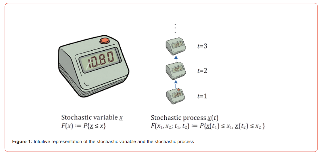
The application of probability theory to real-world phenomena is realized through the concept of the random variable (or stochastic variable), whose definition—both mathematical and intuitive— can be challenging to grasp. Mathematically, a random variable is a function that maps elements of the sample space Ω to real numbers [5]. Figure 1 offers a schematic, intuitive representation of the concepts of a random variable and a stochastic process. A random variable x can be envisioned as a device that produces a random number , with a frequency of appearance equal to F(x), each time a button is pressed. Extending this concept, a stochastic process can be conceptualized as a sequence of such devices—identical in structure if the process is stationary—each generating a random value at a specific, discrete point in time. The fundamental characteristics of a random variable are described by its distribution function, F(x). In the case of stochastic processes, it is necessary not only to know the individual distribution functions of the random variables (the same function if stationary) but also, at minimum, the second-order distribution function, F(x1, x2; t1, t2), which captures the joint behavior of the process at two different times. The Kolmogorov’s axiomatic framework laid the groundwork for modern probability theory and provided a solid mathematical basis for analyzing stochastic phenomena. Stochastic modeling approaches in hydrology can be broadly categorized into three main types:

a. Univariate frequency analysis, used primarily for the estimation of design values;
b. Multivariate or conditional modeling, which addresses the interdependence among multiple stochastic variables; and
c. Stochastic process modeling, aimed at capturing temporal or spatiotemporal variability.

The key milestones and developments within these three categories—particularly as they pertain to applications in both economics and hydrology—are discussed in the following section.

Univariate frequency analysis

Univariate analysis focuses on problems involving a single stochastic variable. In both hydrology and economics, numerous probability distributions—often originally developed with one field in mind—have found effective application in the other. This crossdisciplinary utility highlights the shared statistical foundations of these sciences. A common hidden element in such analyses is the use of plotting positions, which, though often applied implicitly, are fundamental to evaluating how well observed data fit a presumed theoretical distribution.

The Gumbel distribution—a light-tailed distribution with neither an upper nor lower bound—was originally developed in 1941 for modeling extreme values of physical phenomena, particularly for estimating the probability of natural disasters such as flood flows [6]. Over time, its usefulness extended beyond hydrology. In economics, the Gumbel distribution has become a valuable tool for analyzing extreme macroeconomic events. It is now commonly used to estimate the probability of rare but impactful occurrences, such as unusually high inflation rates or severe drops in gross domestic product [7].

The Pareto distribution was first introduced by the Italian economist Vilfredo Pareto in the late 19th century to describe the distribution of wealth within a society [8]. It is a heavy-tailed distribution, reflecting the observation that a small proportion of the population holds a large proportion of the wealth—an insight later popularized as the “80/20 rule.” Beyond economics, the Pareto distribution has found meaningful applications in hydrology. In particular, Papalexiou et al. [9] demonstrated that it provides improved representation of extreme values in observed daily rainfall, making it a valuable tool for modeling hydrometeorological extremes.

In the early 20th century, hydrologists and engineers faced the challenge of designing infrastructure—such as dams, bridges, and culverts—to withstand rare but extreme hydrological events, including floods and intense rainfall. To address this, Hazen [10] introduced a framework for analyzing the frequency of extreme floods based on available discharge observations, including a formula for calculating plotting positions. This method was later refined by Weibull [11]. Today, plotting positions remain fundamental tools—not only in hydrology but also in economics. They are widely used in constructing percentiles and quantilequantile (Q-Q) plots [12], evaluating income inequality [13], and generating empirical cumulative distribution functions such as Lorenz curves and percentile ranks.

Multivariate / Conditional Modeling

This category encompasses applications involving two or more random variables, where the focus lies on analyzing either their joint behavior or conditional relationships. In both hydrology and economics, such modeling is essential for understanding the interdependencies among variables, such as rainfall and runoff, or income and consumption.

In 1959, the concept of a copula was formalized by Abe Sklar, whose theorem demonstrated that any multivariate joint distribution can be expressed in terms of its marginal distributions and a copula that binds them [14]. Copulas began to gain practical traction in finance in the early 1990s, where they were employed to model the joint behavior of asset returns—particularly in the contexts of portfolio risk management and credit risk modeling [15]. Interest in copulas later expanded into hydrology, where they have been applied to understand dependence structures between variables such as temperature and precipitation [16], and to assess the joint impacts of temperature and precipitation extremes on crop yields [17].

An essential application of stochastics—ubiquitous across hydrology, economics, and virtually all data-driven sciences—is regression analysis. Despite its wide applicability and interpretative richness, the mathematical formulation of regression is remarkably straightforward [4]. For a given realization of equal to x, the regression estimates the expected value of the dependent variable through the conditional expectation:

In linear regression, Equation (1) is typically assumed to take the form ŷ = a0 + a1 x, where a0 and a1 are the regression coefficients. In nonlinear regression, the functional form of Equation (1) is explicitly nonlinear, or alternatively, the data may be transformed through a linearization technique to enable the use of linear regression methods.

The range of regression applications in both hydrology and economics is vast. In economics, the doctoral thesis of Koopmans in 1937 [18] established foundational principles for applying regression to time series data, addressing critical issues such as serial correlation and the identification problem in econometric modeling. Shortly thereafter, Tinbergen [19] employed statistical methods and regression analysis to investigate the acceleration principle, further advancing the integration of stochastics into economic theory.

Hydrology adopted regression techniques somewhat later. One of the most prominent applications is in rainfall-runoff modeling, notably exemplified by the work of Nash and Sutcliffe in 1970 [20], who proposed a widely used performance metric based on regression analysis. Another significant application is the reconstruction of hydrological time series, as demonstrated by Hirsch [21] in studies addressing the estimation of missing or unreliable observations.

When the stochastic variable is binary—such as annual floods that cause damage versus those that do not—a specialized form of regression, logistic regression, is used. In this case, the quantity of interest is the conditional probability , which is modeled using the logistic function. The relationship is expressed as:

Hydrology has significantly benefited from the earlier and more extensive use of logistic regression in economics—so much so that foundational hydrological textbooks (e.g., [22]) reference economic literature, such as [23], to introduce and explain the method.

Bayes’ theorem, introduced posthumously in 1763 by Thomas Bayes, has become a foundational principle in statistical analysis across numerous scientific disciplines. In hydrology, Bayesian inference is widely applied to quantify parameter uncertainty (e.g., [24]) and improve predictive performance through techniques such as model averaging [25]. In economics, forecasting models—particularly those dealing with complex financial and macroeconomic time series—often face challenges related to model uncertainty and over-parameterization. Bayesian methods have emerged as a powerful and flexible framework to address these issues [26].

This subsection concludes with a brief overview of the application of machine learning (ML) techniques across the multivariate and conditional modeling approaches discussed above. Multi-layer perceptron (MLP) models have been employed as multiple regression tools, for example, in modeling daily soil evaporation [27]. Refenes et al. [28] demonstrated the advantages of MLPs in financial modeling by comparing their predictive performance with that of traditional regression methods in stock performance forecasting. Notably, logistic regression can be implemented as an MLP architecture in which the output layer employs a sigmoid activation function. In hydrology, Rozos and Dimitriadis [29] showed that integrating logistic regression with a hydrological model significantly enhances the reliability of flood early warning systems. In economics, logistic regression has been widely used for predicting financial failures (e.g., [30]). Beyond MLPs, other ML techniques have found applications in tasks based on regression or conditional probability estimation. These include support vector regression (e.g., [31] in hydrology; [32] in economics), random forests (e.g., [33] in hydrology; [34] in economics), and k-nearest neighbors (e.g., [35,36] in hydrology; [37] in economics).

Stochastic process modeling

Stochastic process modeling is concerned with representing systems that evolve over time or across spatial domains under the influence of inherent randomness. The two primary applications of stochastic process modeling are the generation of synthetic time series and the propagation of uncertainty through complex systems.

Time series generation serves two primary purposes: exploring the uncertainty inherent in a system and enabling short-term forecasting—particularly when historical data are used to initialize the stochastic model. The landmark publication by Box and Jenkins in 1970 [38] formalized the use of autoregressive integrated moving average (ARIMA) models, establishing a comprehensive methodological framework for time series analysis and forecasting. Although autoregressive models appeared in hydrology literature as early as 1977 [39], the widespread adoption of stochastic modeling in the field was gradual. For instance, the seminal textbook Applied Hydrology of Chow published in 1971 [40] provided only a cursory distinction between stochastic and deterministic approaches. It was not until the release of the Handbook of Hydrology in 1993 [41] that ARIMA models received extensive treatment, signaling a broader acceptance of stochastic modeling in hydrology. In contrast, economics embraced stochastic approaches more rapidly; foundational textbooks addressed such models even prior to the Box and Jenkins publication [42]. By 1974, stochastic modeling was sufficiently prevalent in economics to prompt critical evaluations of misuse, such as the influential paper by Granger and Newbold [43], which cautioned against spurious regression results.

A pivotal discovery in the realm of stochastic processes emerged well before their widespread adoption across scientific disciplines. In 1951, H.E. Hurst published his seminal work identifying longterm dependence—also referred to as persistence—in hydrological time series such as river flows and rainfall [44]. This finding has since become foundational in modern stochastic hydrology (e.g.,[45]), influencing how uncertainty and memory are modeled in natural systems. The concept of persistence has also permeated other fields, notably economics, where it is now recognized as a key characteristic in phenomena such as volatility clustering in inflation [46] and temporal clustering in asset price fluctuations [47], wherein periods of high or low values tend to occur consecutively.

A major scientific breakthrough in the field of stochastics occurred with the introduction of the Monte Carlo method in 1949 by Metropolis and Ulam [48]. Closely linked to the quantification and exploration of system uncertainty, this method gained widespread adoption with the advent of computers, which enabled extensive numerical computations. Monte Carlo simulation rapidly became an indispensable tool for uncertainty analysis in both hydrology and economics. Fundamentally, Monte Carlo is a stochastic integration technique used to estimate integrals, such as those arising in the Frobenius–Perron (FP) operator. This operator characterizes the propagation of uncertainty by integrating over the domain defined by the inverse of the system’s governing function. In its simplest form, the FP operator can be expressed as follows to illustrate the principle:

where f_t and f_t−1 are the probability density functions of the stochastic variables x_t and x_t−1, which represent the state of a system at time steps t and t−1.

In hydrology, techniques akin to the Monte Carlo method appeared in unconventional forms decades before its formal introduction by Metropolis and Ulam. Typical applications include the estimation of the variance of skewness from observational data [49], reservoir capacity design based on sets of synthetic time series [50], and the study of uncertainty propagation in simulating the state of simple yet chaotic systems [51]. In economics, Monte Carlo simulation found early use in corporate finance, where probabilistic modeling was employed to assess the risks associated with capital investment decisions [52]. Additionally, Monte Carlo methods were applied in simulation-based approaches to option pricing in the European financial environment [53].

This subsection concludes with the most recent advancements in applying machine learning (ML) to stochastic modeling and uncertainty analysis. In both hydrology and economics, ML has frequently been used to estimate the conditional probability of future values of a stochastic process based on past observations, enabling more accurate forecasting. In hydrology, Minns and Hall [54] were pioneers in employing a multilayer perceptron (MLP) that incorporated past output values as inputs, effectively implementing a recurrent neural network (RNN). Similarly, in economics, Moshiri et al. [55] applied an RNN to forecast inflation. The introduction of long short-term memory (LSTM) networks marked a significant improvement over traditional RNNs, sparking renewed research in both fields. For instance, LSTM has been applied in hydrology to forecast low daily discharge flows [56]. In economics, multiple studies (e.g., [57]) have demonstrated the superior performance of LSTM compared to traditional methods such as ARIMA for economic and financial time series prediction.

The latest breakthrough in ML for modeling conditional probabilities with respect to past values is the Transformer architecture, which underpins powerful large language models. This innovation has attracted considerable attention from researchers in both disciplines. In hydrology, Transformer models have been successfully used for drought forecasting, outperforming previous leading models like LSTM [58]. In economics, secondgeneration Transformer variants such as Informer, Autoformer, and PatchTST have shown remarkable efficacy, especially in scenarios characterized by limited historical data and volatile markets [59].

Finally, for the generation of unconditional synthetic time series that reliably reproduce the first- and second-order distribution functions of a stochastic process, generative adversarial networks (GANs) have proven capable of nuanced replication of the statistical properties of historical financial time series, including persistence [60]. In hydrology, GANs have attracted considerable attention over recent years [61] and have primarily been applied to characterize hydrological structures [62] and predict floods [63]. However, to date, GANs have not been employed for the generation of synthetic hydrological time series.

Hydrology and economics can be seen as twin laboratories for the development, refinement, and application of stochastic methods. Despite the apparent differences in subject matter— natural systems versus human systems—both disciplines share a common need to understand, model, and forecast processes that are inherently uncertain and influenced by complex interdependencies over time. This shared need has led to an exchange of ideas, where advancements in one field have often inspired progress in the other. Historically, many stochastic tools were developed or adopted earlier in economics and only later made their way into hydrology. For instance, regression analysis was formalized and broadly applied in economics decades before it became a staple in hydrological modeling. Econometricians like Tjalling Koopmans and Jan Tinbergen were pioneers in applying statistical methods to time series analysis, paving the way for techniques such as autoregressive models, which were only gradually adopted by the hydrological community in the latter half of the 20th century. Logistic regression, too, found its early applications in financial and econometric contexts before being embraced by hydrologists to improve predictive models, such as those used in flood early warning systems.

Conversely, hydrology has made foundational contributions to the understanding of stochastic processes that have had farreaching implications beyond its own boundaries. A particularly notable example is the work of H.E. Hurst, whose seminal 1951 study on the long-term memory (or persistence) of hydrological time series introduced what is now widely known as the Hurst phenomenon. His findings challenged prevailing assumptions about randomness and independence in time series, prompting significant re-evaluations in both natural and social sciences. Today, the concept of persistence is recognized as a crucial property in economic phenomena such as inflation dynamics and market volatility.

In more recent years, both fields have embraced machine learning and data-driven approaches, often in parallel, with mutual benefits. Techniques like neural networks, support vector machines, and transformers have been independently adopted and tailored to the distinct needs of hydrology and economics—whether forecasting river flows or predicting stock market movements.

In summary, the evolution of stochastics in hydrology and economics illustrates a dynamic and reciprocal relationship. While economics has often led in the early application and development of statistical methods, hydrology has contributed profound conceptual insights—most notably persistence—that have reshaped stochastic thinking across disciplines. Recognizing this interplay not only enhances our appreciation of both fields but also encourages continued collaboration and innovation in tackling uncertainty across the natural and social worlds.

1. Dunham W (1990) Journey Through Genius (1st ed.) John Wiley and Sons.
2. (2025) Ars Conjectandi. Wikipedia, Wikimedia Foundation, United States.
3. Koutsoyiannis D (2024) Stochastics of hydroclimatic extremes - A cool look at risk. 4 ed KALLIPOS, Athens, Greece.
4. Papoulis A (1990) Probability and Statistics. Prentice-Hall, New Jersey, US.
5. Kolmogorov AN (1933) Basic concepts of probability theory. results of mathematics (2), Berlin.
6. Gumbel EJ (1941) The return period of flood flows. The Annals of Mathematical Statistics 12(7): 163-190.
7. Gilli M, këllezi E (2006) An Application of Extreme Value Theory for Measuring Financial Risk. Comput Econ 27: 207-228.
8. Pareto V (1896) Course in Political Economy Professor at the University of Lausanne. F Rouge, Lausanne, France.
9. Papalexiou SM, Koutsoyiannis D, Makropoulos C (2013) How extreme is extreme? An assessment of daily rainfall distribution tails. Hydrology and Earth System Sciences 17(2): 851-862.
10. Hazen A (1914) The storage to be provided in impounding reservoirs for municipal water supply. Transactions of the American Society of Civil Engineers 77(9): 1539-1669.
11. Weibull W (1939) A statistical theory of strength of materials. Ing. Vetensk. Akad Handl 151(1): 1-45.
12. Spasova T (2024) Estimating Income Distributions from Grouped Data: A Minimum Quantile Distance Approach. Comput Econ 64: 2079-2096.
13. Sievertsen H (2024) Introduction to Economic Data.
14. Sklar A (1959) Distribution Functions of n Dimensions and Margins. Publications of the Institute of Statistics at the University of Paris, Paris pp. 229-231.
15. Li DX (2000) On default correlation. The Journal of Fixed Income 9(4): 43-54.
16. Lazoglou G, Anagnostopoulou C (2019) Joint distribution of temperature and precipitation in the Mediterranean, using the Copula method. Theoretical and applied climatology 135: 1399-1411.
17. Alidoost F, Su Z, Stein A (2019) Evaluating the effects of climate extremes on crop yield, production and price using multivariate distributions: A new copula application. Weather and Climate Extremes 26: 100227.
18. Koopmans TC (1937) Linear Regression Analysis of Economic Time Series. Haarlem Netherlands Economic Institute, De Erven F Bohn NV, Netherlands.
19. Tinbergen J (1938) Statistical evidence on the acceleration principle. Economical 5(18): 164-176.
20. Nash JE, Sutcliffe JV (1970) River flow forecasting through conceptual models part I-A discussion of principles. Journal of hydrology 10(3): 282-290.
21. Hirsch RM (1979) An evaluation of some record reconstruction techniques. Water resources research 15(6): 1781-1790.
22. Hirsch RM, Helsel DR, Cohn TA, Gilroy E J (1993) Statistical analysis of hydrologic data. In Handbook of Hydrology (ed. Maidment, D. R.), McGraw-Hill, New York pp. 17(8): 1-17.52.
23. Amemiya T (1981) Qualitative response models: A survey. Journal of economic literature 19(4): 1483-1536.
24. Kavetski D, Kuczera G, Franks SW (2006) Bayesian analysis of input uncertainty in hydrological modeling: 1. Theory. Water Resour Res 42(3): W03407-W03409.
25. Duan Q, Ajami NK, Gao X, Sorooshian S (2007) Multi-model ensemble hydrologic prediction using Bayesian model averaging. Adv Water Resour 30(5): 1371-1386.
26. Koop G, Korobilis D (2010) Bayesian multivariate time series methods for empirical macroeconomics. Foundations and Trends® in Econometrics 3(4): 267-358.
27. Han H, Felker P (1997) Estimation of daily soil water evaporation using an artificial neural network. Journal of Arid Environments 37(2): 251-260.
28. Refenes AN, Zapranis A, Francis G (1994) Stock performance modeling using neural networks: a comparative study with regression models. Neural networks 7(2): 375-388.
29. Rozos E, Dimitriadis P (2023) Synergizing machine learning and hydrological models: Enhancing early warning systems. Eur. Water 83(84): 33-40.
30. Pardeshi B (2022) Logistic Regression Analysis for Prediction of Financial Failure: Evidence from Central Public Sector Enterprises in India. Vision: The Journal of Business Perspective 1(1): 1-8.
31. Raghavendra S, Deka PC (2014) Support vector machine applications in the field of hydrology: A review. Applied Soft Computing 19(6): 372-386.
32. Sermpinis G, Stasinakis C, Theofilatos K, Karathanasopoulos A (2014) Inflation and unemployment forecasting with genetic support vector regression. Journal of Forecasting 33(6): 471-487.
33. Schoppa L, Disse M, Bachmair S (2020) Evaluating the performance of random forest for large-scale flood discharge simulation. Journal of Hydrology 590(6): 125531-125538.
34. Yoon J (2021) Forecasting of real GDP growth using machine learning models: Gradient boosting and random forest approach. Computational Economics 57(1): 247-265.
35. Modaresi F, Araghinejad S, Ebrahimi K (2018) A comparative assessment of artificial neural network, generalized regression neural network, least-square support vector regression, and K-nearest neighbor regression for monthly streamflow forecasting in linear and nonlinear conditions. Water resources management 32(5): 243-258.
36. Rozos E, Koutsoyiannis D, Montanari A (2022) KNN vs. Bluecat—Machine learning vs. classical statistics. Hydrology 9(6): 101-108.
37. Imandoust SB, Bolandraftar M (2013) Application of k-nearest neighbor (knn) approach for predicting economic events: Theoretical background. International journal of engineering research and applications 3(5): 605-610.
38. Box GE, Jenkins GM (1970) Time Series Models for Forecasting and Control. Holden Day, San Francisco, USA.
39. Haan CT (1977) Statistical Methods. ISO Central Secretariat, Geneva, Switzerland.
40. Chow Ven Te (1971) Applied hydrology. McGraw-Hill, New York, USA.
41. Maidment DR (1993) Handbook of Hydrology, McGraw-Hill, Colombia, USA.
42. Theil H, Beerens GAC, Tilanus CG, De Leeuw CB (1966) Applied economic forecasting (Vol. 4). North-Holland Publishing Company, Amsterdam, Netherlands.
43. Granger CW, Newbold P (1974) Spurious regressions in econometrics. Journal of econometrics 2(2): 111-120.
44. Hurst HE (1951) Long term storage capacities of reservoirs. Trans. Am. Soc. Civil Eng. 116(1): 776-808.
45. Koutsoyiannis D (2002) The Hurst phenomenon and fractional Gaussian noise made easy. Hydrological Sciences Journal 47 (4): 573-595.
46. Owyang MT (2001) Persistence, excess volatility, and volatility clusters in inflation. Review Federal Reserve Bank of Saint Louis 83(6): 41-52.
47. Kim S, Eom C (2008) Long-term memory and volatility clustering in high-frequency price changes. Physica A: Statistical Mechanics and its Applications 387(5-6): 1247-1254.
48. Metropolis N, Ulam S (1949) The Monte Carlo method. Journal of the American Statistical Association 44(247): 335-341.
49. Wallis JR, Matalas NC, Slack JR (1974) Just a moment. Water Resour Res 10(2): 211-219.
50. Salas J D (1993) Analysis and modelling of hydrological time series. Handbook of hydrology, In Handbook of Hydrology (ed. Maidment DR) McGraw-Hill, New York pp. 19.48-19.49.
51. Koutsoyiannis D (2010) A random walk on water. Hydrology and Earth System Sciences 14(3): 585-601.
52. Hertz DB (1964) Risk analysis in capital investment. Harvard business review 42(2): 95-106.
53. Boyle PP (1977) Options: A monte carlo approach. Journal of financial economics 4(3): 323-338.
54. Minns AW, Hall MJ (1996) Artificial neural networks as rainfall-runoff models. Hydrol Sci. J 41: 399-417.
55. Moshiri S, Cameron NE, Scuse D (1999) Static, dynamic, and hybrid neural networks in forecasting inflation. Computational Economics 14(5): 219-235.
56. Sahoo BB, Jha R, Singh A, Kumar D (2019) Long short-term memory (LSTM) recurrent neural network for low-flow hydrological time series forecasting. Acta Geophysica 67(4): 1471-1481.
57. Siami Namini S, Namin AS (2018) Forecasting economics and financial time series: ARIMA vs. LSTM. arXiv preprint arXiv pp. 1-19.
58. Amanambu AC, Mossa J, Chen Y H (2022) Hydrological drought forecasting using a deep transformer model. Water 14(22): 3611-3618.
59. Souto HG, Moradi A (2024) Can transformers transform financial forecasting? China Finance Review International p. 1-9.
60. Takahashi S, Chen Y, Tanaka-Ishii K (2019) Modeling financial time-series with generative adversarial networks. Physica A: Statistical Mechanics and its Applications 527(5): 121261-121268.
61. Shen C (2018) A transdisciplinary review of deep learning research and its relevance for water resources scientists. Water Resources Research 54(11): 8558-8593.
62. Cui Z, Chen Q, Liu G, Xun L (2024) SA‐Relay GANs: A novel framework for the characterization of complex hydrological structures based on GANs and self‐attention mechanism. Water Resources Research 60(1): e2023WR035932-e2023WR035938.
63. Do Lago CA, Giacomoni MH, Bentivoglio R, Taormina R, Junior MNG, et al. (2023) Generalizing rapid flood predictions to unseen urban catchments with conditional generative adversarial networks. Journal of Hydrology 618(8): 129276-129279.