Oceanwater Temperature and Salinity from Marine Seismic Data for Weather and Climate Research, the Current State, and Future Possibilities

Distributions of oceanic temperature (T) and salinity (S) are the primary drivers of ocean dynamics [1]. These T and S distributions, in association with the atmosphere-hydrosphere interactions have been studied in relation to the recent climatic variations [2, 3] and developing models for predicting occurrences of the future hurricanes [4].

Physical Oceanographers measure T and S data at sparse locations using disposable instruments such as the eXpendable BathyThermograph (XBT) and Conductivity Temperature Depth (CTD) sensors. These instruments measure T and S with a vertical resolution of about 1 meter. They are, however, sparsely deployed, typically from tens to hundreds of kilometers apart. These T and S measurements from sparse locations, when interpolated in-between to pro- vide the oceanic T and S distributions, are of low lateral resolution and may not be very reliable [5]. Therefore, estimating T and S with higher lateral resolutions than that is obtainable from XBT and CTD measurements is desirable [5],

Moving away from the XBT and CTD, marine seismic data show visible reflections within the water-column. These reflections are due to subtle sound-speed variations of the oceanwater, typically ranging from about 1545 m/s at the sea-level to approximately 1485 m/s to a depth of 1000-1200 m and then staying nearly constant [6]. These sound-speed variations (V) are, in turn, related to the variations of T, S, and pressure (P) via the equation of state [7, 8], given as

Exact expressions for CW(T, P), A(T, P), B(T, P), and D(P) can be found in the references cited above. Note from equation 1 that V is a function of not only T and S, but also the pressure P, which is function of the latitude (⏀) and the depth (z). However, P can be easily calculated [6, 9]. So, if we can estimate V by inverting the marine seismic data, it is possible to start from an initial guess of T and S and compute V using equation 1 and iteratively modify T and S using an optimization (inversion) scheme such that the V computed from T and S satisfactorily matches with the V estimated from seismic inversion. When they match to an acceptable accuracy, we may then conclude that the T and S estimated from optimization is reasonable. Although these T and S estimates from marine seismic data are of lower vertical resolution (~5 meters) than XBT and CTD, their lateral resolution is much higher (25 meters or less). Thus, the high vertical resolution of XBT and CTD in combination with the high lateral resolution of the seismic, can potentially provide high-resolution oceanwater T and S estimates for the weather and climate related research.

In the following, we first provide a brief overview of the current state-of-the-art for estimating V from seismic inversion and discuss the optimization procedure for estimating T and S from the inverted V. Next, we discuss the future possibilities of using recent advances of machine learning to directly estimate T and S from seismic data. Finally, we end with some concluding remarks.

Seismic inversion is a nonunique problem and therefore requires an initial model [10]. The primary reason for this requirement is to ensure that the inversion converges to a meaningful solution, not to an undesired one [9]. In the subsurface exploration of the solid earth, such an initial model at sparse locations are usually available from the well-logs. Interpolating these models at sparse locations along the horizons, interpreted from the stacked seismic data then provides the initial model for the entire area of interest. For the problem of the sound-speed estimation from the water-column reflections, such an initial model can be generated from the XBT and CTD data. However, because of sparse deployments of XBT and CTD sensors, they may not be available, and yet, we would like to obtain an initial sound-speed model for inversion.

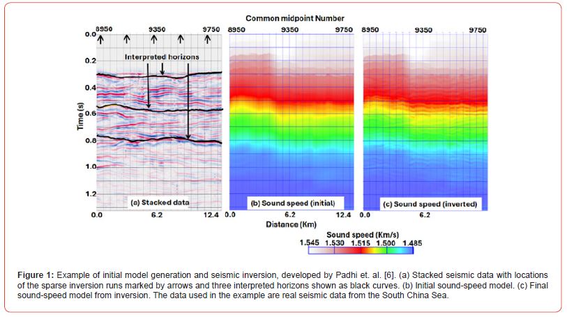
To obtain a reliable sound-speed model in the absence of XBT and CTD data, Padhi, et al. [6] developed a methodology which is illustrated in Figure 1. By carefully running seismic inversion using genetic algorithm (GA) optimization [11-14] at five sparse locations, detailed sound-speed for those locations were first obtained. These locations are marked by arrows on top of the stacked seismic data, shown in Fig.1a. Following these sparse inversions, three horizons, shown as black curves in Fig.1a, were interpreted and the inverted models at sparse locations were laterally interpolated in-between these interpreted horizons to obtain an initial model for the entire seismic line. This initial model is shown in Fig.1b. Note that instead of using the detailed sound-speed models from the sparse inversion runs, their smoothed versions were used in these interpolations. Finally, starting from the initial sound-speed models for each common midpoint (CMP) location shown in Figure 1b, Padhi, et al. [6] inverted those locations and obtained detailed sound-speed model for the entire seismic data, shown in Figure 1c.

The process of the initial model generation and inversion illustrated in Figure 1 although worked well on the real marine seismic data from the South China Sea, it suffers from some difficulties for practical implementation. First, the GA-based inversions at sparse locations are computationally demanding and require a lot of technical expertise. In the two-dimensional (2D) example shown in Figure 1 sparse inversions at five locations were adequate. For three-dimensional (3D) seismic data, a lot more such inversions would be necessary, which could be prohibitively expensive. Second, interpreting horizons from stacked seismic data is prone to human errors. Lastly, by comparing the initial model (Figure 1b) and the final inverted model (Figure 1c), it is evident that the imprint of the initially picked horizons is propagated across the inverted model. If additional horizons were picked for interpolation, it is likely that the inverted model would look different from the one shown in Figure 1c. Thus, the inverted model tends to be biased by the interpreted horizons and it is desirable to obtain a bias-free inversion result in which the imprint of the interpreted horizons are not propagated across like the example of Figure 1.

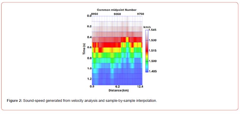
To obtain bias-free inversion, an attribute-guided method to generate the initial model has been recently developed, which does not require any sparse inversion runs nor does it require any horizon- guided interpolation [9, 15]. In this attribute-guided approach, an initial model is first generated via an automated velocity analysis [16, 17] at every 50th CMP location and then laterally interpolating them. This lateral interpolation is performed purely on a sample-by-sample basis, not guided by any interpreted horizon. Figure 2 shows this initial model for the same South China Sea data, shown in Figure 1. Using the initial model of Figure 2, prestack seismic data were then compensated for geometrical spreading loss, corrected for normal moveout (NMO), and stacked [16, 17]. The stacked seismic data obtained from this procedure was identical to the one shown in Figure 1a and therefore not shown.

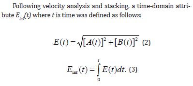
In equation 2, A(t)represents stacked seismic data, and B(t) is computed from A(t) as follows:

1. Fourier transform A(t) from time to frequency (⍵) domain to compute A(⍵).

2. For each sample of A(⍵), interchange the real and imaginary parts to obtain B(⍵).

3. Inverse Fourier transform B(⍵) to time domain and take its real part as B(t).

Figure 3 is the cross-plot between the computed attribute E^int(t) and the sound-speed obtained from the velocity analysis and lateral interpolation (Figure 2) for the same five locations that are marked with arrows in Figure 1a. The plotted points in this Figure are shown as black dots. In addition, a best-fit polynomial through those points is computed and shown as red curve in Figure 3. The equation represented by this best-fit polynomial was found to be:

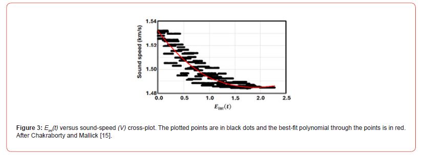
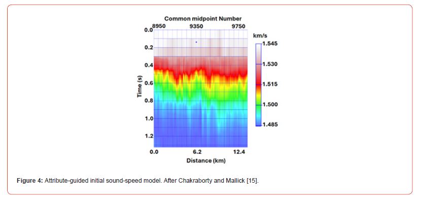
with a R₂ value of 0.8741 [15]. Using equation 4, the soundspeed for the entire seismic line was then computed directly from the attribute E_int(t) and is shown in Figure 4.

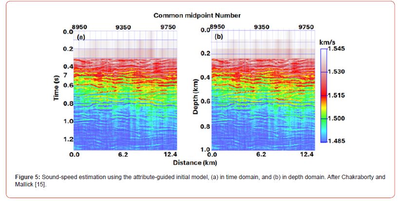
Finally, using the attributed-guided sound-speed model of Figure 4 as the initial model, the entire seismic data were inverted, and the results are shown in Figure 5 in both time (Figure 5a) and depth (Figure 5b) domains. From a visual comparison of the inverted model in time domain (Figure 5a) with the stacked seismic data (Figure 1a), note that although our initial model of Figure 4 did not have any horizon information, the inversion result is in perfect agreement with the reflection boundaries in the stacked seismic data. Therefore, the attribute-guided initial model (Figure 4) is not prone to any bias to which the horizon-guided initial model (Figure 1b) is subject to. Additionally, this attribute-guided approach is fully automated and does not require any sparse inversion runs. We thus believe that the attribute-guided approach can be used for estimating V from marine seismic data on a routine basis.

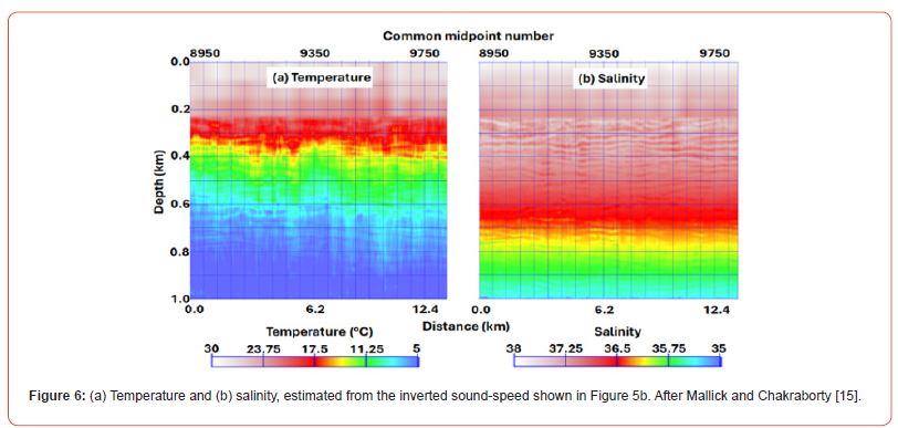
Following the estimation of the sound-speed (V), the next step is to estimate the temperature (T) and salinity (S) from V. To do so, Chakraborty and Mallick [15] started from an initial T and S model and used the Adaptive Moment Estimation (ADAM) optimization method [18] to simultaneously estimate T and S from V. The exact methodology for this ADAM optimization for T and S estimation can be found in the reference cited above, and in Figure 6 we provide the results of these estimates. Like attribute-guided seismic inversion, the ADAM methodology for T and S estimations are also fully automated, and therefore applicable to marine seismic data on a routine basis.

The T and S estimations, discussed above used a two-step process. In step-1, the seismic data were inverted to obtain V (Figure 5) and in step-2, T and S were estimated from V (Figure 6). Although we argued that the entire process is fully automated and can be used on a routine basis, we must note that the seismic inversion for estimating V is computationally demanding [15]. It is therefore worthwhile to investigate if the overall computational efficiency of the method could be improved.

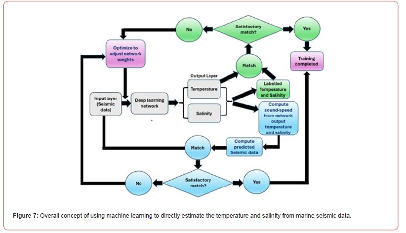
Use of artificial intelligence (AI), specifically machine learning (ML) recently revolutionized almost all fields of applied science and engineering, including geosciences. In Figure 7, we provide our vision of how ML could potentially convert the two-step approach to a single step of directly estimating T and S from seismic data and improve overall computational efficiency.

Both conventional supervised learning using labelled data and supervised learning using physics-informed machine learning (PIML) is outlined in Figure 7. For convenience, we used different colors to identify different modules in the architecture shown in this Figure. Fundamental ML steps using a deep neural network are shaded in light gray, the supervised learning components using labelled data are shaded in green, and the PIML components are shaded in blue. Finally, the components that are used by both supervised learning from labelled data and PIML are shaded in purple.

As shown in Figure 7, the input seismic data from the input layer are fed to a deep learning architecture such as a convolutional neural network, which will directly output T and S. For learning using labelled data, the T and S output form the network will be compared with their corresponding labels to compute the loss function and fed to an optimization method such as ADAM for adjusting weights. For PIML based learning, we can compute the soundspeeds from the T and S output from the network using equation 1 and then compute synthetic (predicted) seismic data. By comparing these synthetic seismic data with their corresponding real seismic data from the input layer, we can then compute the loss function and feed to the optimizer for weight adjustment. By using a selected set of training and validation data, computing the optimum network weights, and then applying to the entire data is expected to be a computationally efficient way to directly estimate T and S from marine seismic data.

We provided an overview of a two-step inversion method to estimate the oceanwater temperature and salinity from marine seismic data. We also provided a vison of how this two-step process can be converted to a single step using machine learning and improve overall computational efficiency. Lateral resolution of the estimates of temperature and salinity from marine seismic data are much higher than those obtainable from XBT and CTD. Therefore, marine seismic data could potentially be used for future weather and climate related research.

We acknowledge the use of computational resources at the Advanced Research Computing Center (ARCC) of the University of Wyoming (https://doi.org/10.15786/M2FY47) and the NCAR Wyoming Supercomputing Center provided by the National Science Foundation and the State of Wyoming and supported by NCAR’s Computational and Information Systems Laboratory (https://doi. org/10.5065/D6RX99HX).

There is no conflict of interest.

1. Thorpe SA (1967) The Turbulent Ocean. Cambridge University Press.
2. Meredith MP, King JC (2005) Rapid climate change in the ocean west of the Antarctic Peninsula during the second half of the 20^th Geophysical Research Letters 32: L96104 1-5.
3. Durac PJ, Wijffels, SE, Matear RJ (2012) Ocean Salinities Reveal Strong Global Water Cycle Intensification During 1950 to 2000. Science 336: 455-458.
4. Bender MA, Knutson TR, Tuleya RE, Sirutis JJ, Vecchi GA, et al. (2010) Modeled Impact of Anthropogenic Warming on the Frequency of Intense Atlantic Hurricanes. Science 327 (5964): 454-458.
5. Smith DM and Murphy JM (2006) An objective ocean temperature and salinity analysis using covariances from a global climate model. Journal of Geophysical Research 112(C02022): 1-19.
6. Padhi A, Mallick S, Fortin W, Holbrook WS, Blacic TM (2015) 2-D ocean temperature and salinity images from pre-stack seismic waveform inversion methods: an example from the South China Sea. Geophysical Journal International (202): 800-810.
7. Chen CT, Millero FJ (1977) Speed of sound in seawater at high pressures. Journal of the Acoustical Society of America 62(5): 1129–1135.
8. Fofonoff P, Millard RC Jr (1983) Algorithms for computation of fundamental properties of seawater, UNESCO Tech Pap In Mar Sci No. 44: 53.
9. Mallick S, Chakraborty D (2022) Prediction of the ocean water sound speeds via attribute-guided seismic waveform inversion. Geophysics 87: U67-U79.
10. Tarantola A (1987) Inverse problem theory and methods for model parameter estimation, SIAM (Society of Industrial and Applied Mathematics), ISBN: 978-0898715729.
11. Mallick S (1995) Model-based inversion of amplitude-variations-with-offset data using a genetic algorithm. Geophysics 60: 939-954.
12. Mallick S (1999) Some practical aspects of prestack waveform inversion using a genetic algorithm: An example from the east Texas Woodbine gas sand. Geophysics 64: 326-336.
13. Mallick S, Adhikari S (2015) Amplitude-variation-with-offset and prestack waveform inversion: A direct comparison using a real data example from the Rock Springs Uplift, Wyoming, USA. Geophysics 80: B45–B59.
14. Pafeng J, Mallick S, Sharma H (2017) Prestack waveform inversion of three-dimensional seismic data — An example from the Rock Springs Uplift, Wyoming, USA. Geophysics 82(1): B1-B12.
15. Chakraborty D, Mallick S (2024) Estimation of Temperature and Salinity from Marine Seismic Data—A Two-Step Approach. Journal of Marine Science and Engineering 12(3): 471.
16. Yilmaz Ö (1987) Seismic data processing, Society of Exploration Geophysicists, ISBN: 978-0931830402.
17. Yilmaz Ö (2001) Seismic data analysis: Processing, inversion, and interpretation of seismic data, Society of Exploration Geophysicists, ISBN: 978-1560800989.
18. Kingma DP, Ba JL (2014) ADAM: A method for stochastic optimization. arXiv: 1412.6980.