Correlated Time Series Modeling of Carbon Emissions and Global Temperature Fluctuations

Introduction

The drastic increase in global temperature is an increasingly publicized phenomenon with far reaching implications. While temperatures can deviate naturally year to year, the United Nations International Governmental Panel on Climate Change has concluded that the change (a general warming trend) documented over the past 100 years is unprecedented within the past millennia. Further, the panel finds it ”extremely likely” that human activity is a causal link in this process and that this warming trend poses significant danger for our society [1]. Past estimates have demonstrated that the global temperatures, on average, have risen about 2 degrees Celsius with projections as high as 4 degrees Celsius within the century. Such drastic increases in global temperatures can result in massive detrimental implications to ecosystems worldwide [2]. Arctic Ocean levels, costal city infrastructure, agricultural methodology, water usage, worldwide ecosystems, and migration patterns are just a few of the potential arenas in need of adaptation in an ever warmer world [3]. This phenomenon of global warming is often purported to be correlated with rising carbon emissions. If so, this would underscore the necessity to find alternative fuel sources that do not necessitate emitting carbon.

Historically carbon emissions have been modeled through Lagrangian transport models. The Lagrangian model for carbon emissions is

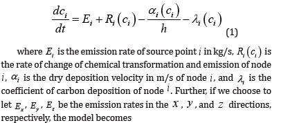
Please [4]. While this model carries insight in its predictive capability, the intuition can be expanded to make a more dynamical model capable of incorporating seasonally fluctuating trends and easily manipulated in the presence of future human positive intervention.

However, this analysis of carbon emissions would be fairly vacuous if not shown in relation to its effect on global temperatures. First consider the data set itself. Previous literature has shown that a scaling factor can be applicable to temperature fluctuations among differing geographic areas. Insofar as temperature measurements are made near the earth’s surface, a power-law scaling with scaling exponent of α = 1 over oceanic surfaces, α =0.5 over continental surfaces, andα =0.65 over transition regions is deemed appropriate [5]. This finding motivates the intuition behind scaling global temperature data, as is done in the NASA data set. Moving beyond the data set itself, short-term correlations in global temperature and meteorological records are often modeled through low-order autoregressive functions (such to the AR-1 model implemented here). The dynamics of which can be taken to obey a first degree ordinary differential equation given by

where ∈(t ) denotes uncorrelated Gaussian noise, and a₀ ,a₁ are constants [6]. Here again, the past precedence using autoregressive functions as adaptive methods to expand upon differential equation models motivated the intuition to do likewise in this study. However, this model will be distinguished by explicitly comparing not only global temperatures with meteorological data generally, but specifically with carbon emissions in an attempt to better isolate the share of environmental deterioration attributable to CO₂.

Thus, it is the aim of this paper to analyze the extent to which carbon emissions, in conjunction with global temperatures, are rising and discuss policy implementation applicable to the findings.

Data

We use two datasets to demonstrate our method and make implementations.

Mauna Loa data set

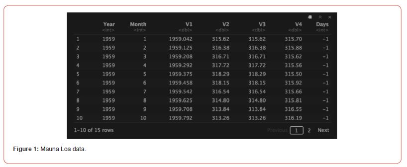
The data on global carbon emissions was garnered from the Earth System Research Laboratory [7]. It was collected via a carbon emission detection system atop Mauna Loa Island in Hawaii. It is worth noting that where will be some seasonal patterns in the data that do not necessarily reflect discrepancies in carbon emissions (this ambiguity will be included in and differentiate our methodology) but rather fluctuations in plant life available to absorb carbon dioxide on Mauna Loa. The variables in the data set are as follows: ”year” ranging from 1959 to 2018, ”month” ranging from 1 to 12 (with 1 signifying Jan. and 12 signifying Dec.) ”V1” being a time variable with a decimal representation of the year and month, ”V2” being monthly average carbon emissions in water-vapor-free-air (measured in parts per million by volume), ”V3” being an interpolated measure that provides estimates for missing observations in V2, V4 being a seasonal correlation trend computed using a moving average of the seven adjacent seasonal cycles centered on the month to be corrected, and ”days” which denotes the number of days included in that month’s mean (this count began in 1974, so -1 is used to denote an unavailable variable before that time period). For example, V2, row 230 represents the carbon emissions on January 22, 1978. Part of the data is shown in Figure 1 table below.

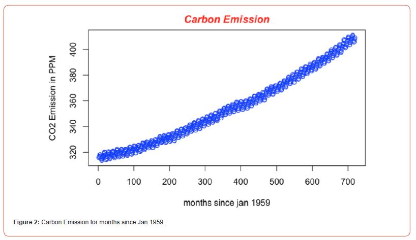
A subset of the data is given in Figure 2 to visually show the trend as index of observations gets bigger.

Global Temperature Fluctuations

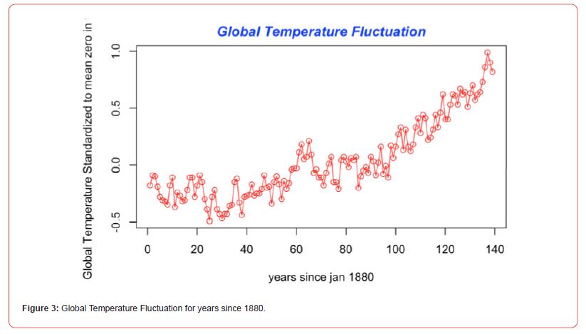
The global temperature fluctuation data set was acquired through the National Aeronautics and Space Administration [8]. This data depicts global annual mean temperatures in degrees Celsius from 1880-2018. The variables are ”year” (from 1880- 2018) and ”temperature” in degrees Celsius scaled such that the time period of the 1950s are mean zero. For example, row 135 signifies the average global temperature in 2013 normalized around the 1950s.

Part of the global temperature fluctuation data is displayed in Figure 3 named ” Global Temperature Fluctuation for years since 1880” to visually show the trend.

Statistical Application

We will demonstrate our method on the two datasets in this section.

Mauna Loa data

For the purposes of this paper, the model for carbon emissions will be derived from a general linear

model

Plots of the data reveal a curvilinear pattern, so a quadratic trend will be included. Further, if one examines the data on a short time interval, a seasonal trend becomes apparent. Thus, fitting a harmonic

sine and cosine wave seem appropriate. Hence, the model is given by,

Global Temperature data

Similarly, the global temperature model will be derived from a general time series model,

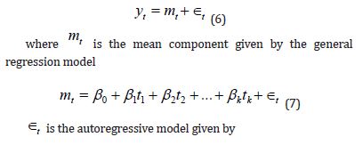
After considering the general pattern of the data with some curvilinear pattern, the regression was fit with a linear and quadratic trend. That is, the model given by

Next, a first order autoregressive model will be implemented. It is given by

Quickly, we do not mean to be too flippant in how we determine the p for our AR(p) model, but given various approaches, from description length criterion to information-theoretic criterion, to simply having computational packages like R handle this decision making process [7, 9] , each giving various differing conclusions, we decided to defer to a convention.

Conclusion

Carbon emissions are increasing in time with not just merely a linear but a quadratic trend. It is worth noting that our model fit a harmonic seasonal trend as well. While this seasonal trend was significant, it is unclear weather carbon emissions actually fluctuate with seasons or if this is actually resulting from fluctuations in organic life surrounding Mauna Loa. Trees intake carbon and will decrease readings in the surrounding area, so when trees are in season, we could expect to see a correlated decrease in carbon. furthermore, throughout the course of this paper, we have derived a predictive model for global warming given by

95% confidence intervals were used to conclude that the β₀, β₁, ,β₂ are significant. Given the quadratic trend is positive this would indicate that global temperatures are rising with, at least, a significant quadratic trend. This model was then used to forecast up to five years from the current time (note the model can be used with decreasing accuracy to forecast even further into the future). Moreover, we have provided first order autoregressive prediction intervals given by

, for the five forecasts made. The intuition gained from the combined results is a similar quadratic trend existing in both time series, which would support the notion that global warming is increasing in correlation with carbon emissions. Future work could include fitting an exponential trend to see if the emissions and/or temperatures are rising even more substantially as well as refining the technique by which one decides on the power of the AR(P) polynomial. The practical implications of these findings are extremely non-trivial. Such marked increases in carbon emissions is hypothesized to cause analogously increasing world temperatures. This substantial global warming can result in the deleterious effects on the polar ice caps. This, in turn, has implications on both the species native to that area as well as species world-wide that are affected by rising ocean tides. These findings should underscore the necessity to cultivate alternative fuel methods and decrease dependence on carbon based fuels. It is worth noting that this would also necessitate future work in the practical implications of a society utilizing primarily electric engines. Such implications include practical concerns of availability of charging ports, financial burden on varying socioeconomic states, and potential market fluctuations in changing demand for resources. Policy recommendations include a carbon tax. A carbon tax, currently suggested at the rate of at least 15 dollars per ton of CO₂ emitted, is the least distortionary mechanism by which we can feasibly reduce carbon emission from 400 ppm to 350 ppm in a reasonable interval of time. That is to say, this tax would be the least detrimental to economic incentives already in place to stimulate domestic and global economies, yet would also provide necessary compulsion to adequately reduce carbon emissions [?]. That said, it is worth noting that is imperative to consider analogous taxes on other harmful emissions, as to prevent disproportionate burden of taxation placed on carbon emissions relative to chlorofluorocarbons. Insofar as this would discourage one emission more than others, this distortion would not be conducive to economic growth or environmental sustainability.

Acknowledgment

I would also like to thank the reviewers for their time.

Conflict of interest

There is no conflict of interest.

References

 

1. New M, Liveman D, Betts R, Anderson K (2011) Four degrees and beyong: the potential for a global temperature increase of four degrees and its implications. Philosophical transactions of the Royal Scociety, 369: 1934
2. Borgeerson SG (2008) Arctic meltdown-the economic and security implications of global warming. Foreigh Affairs 87(2): 63-77
3. Sundarakani B, De Souza R, Goh M, Wagner SM, Manikandan S (2010) Modeling carbon footprints across the supply chain. International Journal of Production Economics 128(1): 43-50.
4. Fraedrich K, Blender R (2004) Scaling of atmosphere and ocean temperature correlation in observations and climiate models. Physical review Letters 90(10):108501.
5. Kiraly A, Janosi IM (2002) Stochastic modelling of daily temperature fluctuations. Physical Review E 65(5): 051102.
6. Pieter Tans, NoAA/ESRL and R.Ralph Keeling, Scripps Institution of Oceanography
7. Gistemp Team (2019) GISS Surface Temperature Analysis (GISTEMP), version 4. NASA Goddard Institute for Space Studies. Dataset accessed 20YY-MM-DD. Lenssen N, G Schmidt, J Hansen, M Menne, A Persin, et al. (2019) Improvements in the GISTEMP uncertainty model. J Geophys Res Atmos 124(12): 6307-6326.
8. Pearse D (1991) The Role of Carbon Taxes in Adjusting to Global Warming. The Economic Journal 101(407): 938-948.
9. Poterba JM (1991). Tax plicy to combat global warming: on designing a carbon tax (No. w3649). National Bureau of Economic Research.