Scalable Unsupervised Feature Selection for Quantitative Biological Data Using Mixture Models

Supervised and unsupervised machine learning algorithms have been extensively applied in medical and epidemiological settings [1,2]. A long-pursued goal in medical research is the development of statistical approaches to identify and model key features associated with disease phenotypes, as well as to identify patient subgroups which explain observed heterogeneities in complex diseases [3]. Supervised learning approaches including tree-based methods such as random forests [4], generalized boosted regression models [5] and parametric regression models such as the least absolute shrinkage and selection operator, otherwise known as LASSO [6], are frequently used approaches which have been applied to identify key features pertaining to complex diseases and medical applications [7,8]. Alzheimer’s disease (AD) is a complex neurological disorder and is the most common form of dementia with no known cure. For this reason, extensive research is aimed at early detection, and establishing a better understanding of the biological, morphological brain features, demographic and lifestyle factors associated with the disorder.

One of the key and earliest biomarkers of AD is the deposition of beta-amyloid (β-A) protein within the cortex tissue, which is most accurately measured by Positron Emission Topography (PET) imaging. As the increase in (β-A) can occur up to two decades in advance prior to the onset of cognitive symptoms, the identification of key brain cortical regions which are affected by the gradual accumulation of A prior to or in the early stages of the disease remains difficult to identify [9]. Supervised statistical approaches have been vital to identify key features associated with AD in small- and large-scale clinical data sets. For example, the work by [10] utilized RF to detect individuals who were susceptible to becoming A accumulators using cerebrospinal fluid, demographic and cognition measurements. In a large-scale analysis of single nucleotide polymorphisms associated with AD, [11] applied LASSO regression using specific screening rules to analyze millions of potential features to find a potential genetic link to AD. See [12] for further examples of supervised and unsupervised machine learning applications in medical imaging related to AD.

An underlying requirement for all supervised approaches is their dependence on the known response. In the instance of early AD detection research, it is possible for pre-symptomatic individuals to have positive disease pathology markers prior to clinical diagnosis. In the instance when disease groups remain unknown, unsupervised algorithms become a popular alternative. Unsupervised clustering algorithms such as k-means clustering [13], are frequently used to identify hidden sub-populations by dividing the observations into groups or clusters by minimizing the within cluster variation. However, unlike their supervised algorithm counterparts, one of the main task of unsupervised methods is to group all observations into clusters and not facilitate feature selection, which is often available in supervised approaches. An alternative approach to identify potentially hidden disease groups as well as feature selection with respect to these groups is needed in order to provide preliminary and exploratory insight into complex diseases.

Furthermore, as the scale of medical data can range from small to quite large [14,15], a desirable feature for such an approach is to be scalable to facilitate the analysis of a large scope of features. Methodologies which are scalable are a desirable trait in large medical data applications such as bioinformatics [16], epidemiology [17] and medical imaging [18] to name a few. In this work we propose an unsupervised feature selection and prediction algorithm, which uses Gaussian mixture models to identify and classify hidden disease and non-disease groups, and rank features by order of importance. We term this new approach FSPmix. FSPmix first identifies features which supports the presence of two hidden disease and non-disease groups, and then classifies each observation into one of three groups: A or B to denote disease or non-disease groups respectively, as well observations which remain unclassified (group C) if their observed value falls within the group separation criteria. Our FSPmix algorithm then ranks selected features by order of importance, in a similar manner to supervised alternatives such as RF. This enables the FSPmix to aggregate hidden disease group detection and combines classification (like unsupervised approaches) with feature selection (like supervised methods).

For a thorough assessment of this work, we perform two simulation studies and compare the performance of the FSPmix with both the known solution, and other well-known supervised and unsupervised algo-rithms. In a similar manner we apply the FSPmix on case study data, to identify hidden groups of those with or without amyloid burden and again compare our results to several supervised and unsupervised approaches. The layout of this paper is as follows. The Data Section describes the motivating case study considered in this work, which is the Alzheimer’s Disease Neuroimaging Initiative (ADNI) study, [19]. Section titled ‘FSPmix unsupervised feature selection and prediction using mixture models describes our unsupervised feature selection algorithm including our approach for validating the methodology via a simulation study and comparison with three supervised feature selection algorithms (RF, LASSO and GBM) and classification predictive performance compared with an unsupervised classification (k-means) method. ‘Results Section pertains to simulated and case study results and and concluding remarks of our work is presented in the Discussion Section.

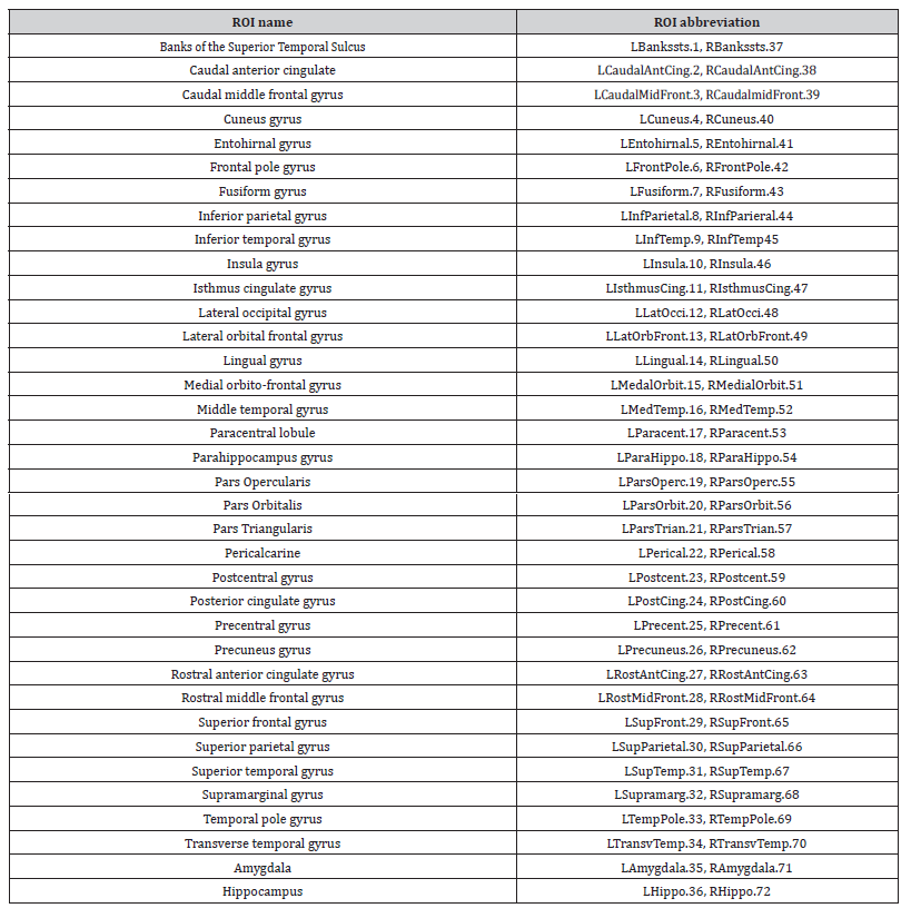
In this paper, we analyze both simulated data as well as data from the ADNI study. Data used in the preparation of this article was obtained from the ADNI database (adni.loni.usc.edu). The ADNI study was launched in 2003 as a public-private partnership, led by Principal Investigator Michael W. Weiner, MD. The primary goal of ADNI has been to test whether serial magnetic resonance imaging (MRI), PET, other biological markers, and clinical and neuropsychological assessment can be combined to measure the progression of mild cognitive impairment (MCI) and early AD. In this work we used florbetapir PET neuroimaging to measure the amount of A protein by the standardized uptake value ratio (SUVR) at the region of interest (ROI) level defined by Desikan atlas and included the amygdala and the hippocampus ROIs. Refer to [20,23] for further description of ADNIs image processing, cerebro-spinal fluid (CSF) collection and additional ADNI protocols. See Appendix A.1 for a full list of ROIs used in this work.

Our FSPmix algorithm was applied to 72 SUVR ROI estimates on a subset of 853 individuals at baseline, which include 266 cognitively normal (CN), 440 MCI 147 AD participants. While the FSPmix is an unsupervised algorithm, in order to compare its feature selection capability with other supervised approaches, we define the following disease and non-disease groups: participants with a global SUVR value of less than 0.8724 and a CSF A 42 value greater than 192 pg/ml were considered to be pathology negative (Response = 0), while participants with a global SUVR value of greater than 0.8724 and a CSF A 42 value less than 192 pg/ml were considered to be pathology positive (Response = 1).

FSPmix: Unsupervised Feature Selection and Prediction Using Mixture Models

Our FSPmix algorithm can be formulated by the pseudocode shown in Algorithm 1. Our approach utilizes a combination of mixture models models in-conjunction with bootstrapping allowing our semi-parametric approach to handle a range of continuous feature characteristics and classify, where possible each feature into two groups: disease and non-disease groups.

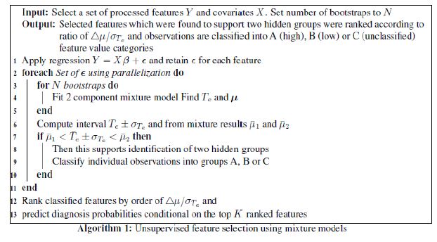
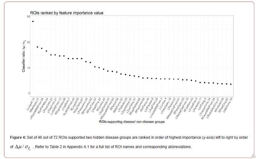
We now describe in detail each of the steps. Once selected features, preferably with the highest variation, are chosen and processed as described in Section 4.3, the first step of Algorithm 1 is to fit a simple linear regression for each feature (Y) in order to take into account the potential variation explained by confounding covariates (X ) of the form Y = Xβ +ε. This is particularly important when considering features which are diagnosis specific, for example, AD individuals in general have accumulated large quantities of amyloid deposition compared to MCI individuals. The residuals of the model (ε ) are retained for each feature and used in the subsequent step. Step 2 of Algorithm 1 utilizes parallelization in order to reduce computational time. This is particularly useful in order to scale up our algorithm to accommodate for large data sets. For each set of feature residualsε , N bootstraps are performed which sampled the data with replacement, and a two-component mixture model of the form.

is fitted. Expression (1) includes two weights with satisfyingProbability densitiesandare Gaussian distributions with parametersμ and σ² respectively. To implement, model g(ε ) is estimated using normalmixEM function from the mixtools R package [24].

The intersection of both Gaussian distributions, e T , is estimated and the component means 1 2 (μ₁,μ₂)are retained for each bootstrap. In order to avoid label switching problem [25] in our computations, we define the component means such that μ₁ < μ₂. While there can be more than one intersection between two Gaussian distributions, our intention is to find the intersection between the two component means as a measure of separation between the two groups. The difference of the log-densities in (1) becomes a quadratic form, and after algebraic manipulation the value of e T is found by finding the roots of the quadratic in the real domain. Over all bootstrap samples for every feature, the them(Te )and standard deviationare retained and used to determine the intervalas shown in Step 6 of Algorithm 1. The mean of the component meansis also computed. By bootstrapping each feature, we attain an estimate on the variation of the separation value e T ; for further information on bootstrap approaches see [26].

Step 7 of Algorithm 1 utilizes the information from Step 6 and classifies each feature as potentially having two hidden groups if the conditionμ is satisfied. This suggests that the difference in the meaning of the mixture component means is substantial enough to strongly support the presence of two groups in a particular feature. For those features which support two hidden groups, observations are classified into either group A denoting lower feature values, group B denoting higher feature values or group C, which are those observa-tions which remain unclassified. In Step 9 of Algorithm 1, an observation is assigned to group A if their value is less thanikewise an observation is assigned to group B if there value is greater thanObservations whose value lies in the range ofare closed as group C and they are considered not to fit to either group A or B. As the algorithm in this work is intended for exploratory purposes, a conservative approach is taken on both identifying which features support two hidden groups, as well as the prediction of each observation groups (A, B or C). This is particularly useful in large data settings where potentially thousands of features could be explored and not all predicted observations easily align into groups A or B.

Steps 12 and 13 of Algorithm 1 pertain to two further analyzes of features which are conditional on their predicted classification of groups A, B or C. The first analysis pertains to ranking all classified features in order of their importance, defined as the separation magnitudeis the difference of means of the component means) which is divided by the standard deviation of the separation interval, Te σ . Large values of the ratio / Te Δμ σ denote that there is a large difference of mean of the component means and/ or Te σ is substantially small. This suggests a particular feature strongly supports two distinct and welldefined groups (A and B) which also results in a small number of observations in group C. On the contrary at the other extreme, if the ratio / Te Δμ σ is small, then this is due to either a small difference in the mean of the component means and/ or a large value of Te σ . Features with small / Te Δμ σ values denote poorly separated groups A and B and as a result tend to have many observations in group C. The second post-analyze pertains to determining weighted predictive disease probabilities based on the top K features as ranked by the order of importance.

The quasi-gold standard (comparative feature) is the feature with the highest importance value / Te Δμ σ and the predictive values (groups A and B) of this feature are then used to compare with group predictions for each of the top K −1features, where the value of K > 2is determined by the user. For example, if 10 out of 100 features were shown to have very large importance values, then the user may wish to investigate how well the predictive disease and non-disease (A and B) groups align with the quasi-gold standard (top ranked feature). Each predicted observation for the top K −1 features is assigned a probability value of zero if an observation in the quasi-gold standard feature and feature of interest is predicted to be in group A. A probability of 0.5 is assigned if there is a mismatch of group A and B classification between the quasi-gold standard and a feature of interest, and finally an observation is assigned a probability of one if the predicted observation in both the quasi-gold standard and feature are both in group B. The average of these value are taken for each observation, to get a weighted probability on how well they correspond to group A (if many of the K −1 features support this predictive value, then majority of the probabilities will tend towards a predicted probability of zero) or alternatively, how well they support a prediction group of B, then these weighted probabilities will tend towards one.

Algorithm 1 was implemented in R using statistical packages mixtools, reshape2 and dplyr. All visualizations of simulated and real data analyze used R package ggplot2. Our feature selection algorithm is available as an R package FSPmix which is available in the GitHub (https://github.com/MarcelaCespedes/FSPmix). In order to rigorously assess the performance of the FSPmix in terms of performance and scalability in a controlled setting, we performed two simulation studies. The scope of simulation study I is to assess the predictive performance of FSPmix on a small set of simulated data which is representative of a wide range of real life like scenarios and includes simulated features which are easily identified as well as challenging features. For comparison with other well-known supervised and unsupervised algorithms, in simulation study I the predictive performance of FSPmix was compared to k-means clustering (unsupervised classification), and the feature selection from FSPmix was compared to three supervised alternatives, RF, LASSO and GBM. The scope of the second simulation study is to assess its Parallelized workflow performance on a large set of synthetic data and determine whether FSPmix is a scalable algorithm.

Simulation Study I

To assess the performance and further validate the FSPmix approach in a controlled setting we conducted two simulation studies. The aim of the first study was to assess the sensitivity and specificity of the FSP algorithm on 20 simulated normalized features as shown in Figure 7 in Appendix A.2. Ten left skewed features were simulated with initial groups far apart (Feature 1) and slowly increasing the overlap of the two groups to a complete overlap by Feature 10. Similar approach was undertaken for the right skewed features, with Feature 11 having the best separated groups, and Feature 20 pertaining to distributions which were overlapping. Data was generated from univariate Gaussian distribution with different means and variance values. A further assessment on the performance of the FSPmix compared the importance ranking of simulated features to those of the three supervised approaches: RF, LASSO and GBM. The FSPmix sensitivity and specificity were assessed over all 20 simulated features, as shown in Figure 1.

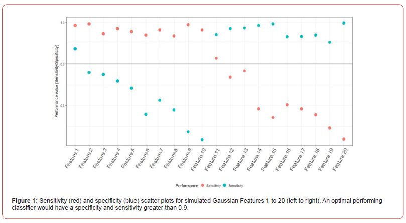
True positive classifications denoted by group A (sensitivity) were summarized as the percentage of classifications which were correctly identified. Likewise, true negative rate (specificity) was summarized by the proportion of group B classifications that were correctly identified by FSPmix. A binary classifier which has perfect recovery of the solution will have both sensitivity and specificity percentages close to one, and alternatively a poor classifier will have these percentages close to zero. In general, binary classifiers will have a trade-off between optimal specificity and sensitivity. As expected, the FSPmix has optimal performance at simulated Features 1 and 11, with both sensitivity and specificity greater than 0.9. The performance of the FSPmix begins to drop as the groups become increasingly overlapping, with the worst performance observed as Features 10 and 20 (the highest overlapping synthetic features). We note, that due to the nature of the classification of groups (A or B) as described in Section 3, depending on whether the data is left or right skewed, the FSPmix will show either consistently high or low sensitivity and specificity, favoring the set of observations from the mixture component with the lowest variance.

The predictive performance of the FSPmix was compared to that of k-means clustering (with k = 2 clusters) on the same simulated data, refer to Figure 9 in Appendix A.2 for full results across all 20 features. While k-means clustering showed near perfect either sensitivity or specificity depending on whether the feature was left or right skewed respectively (similar to the FSPmix results), the alternative specificity or sensitivity value for each feature was lower than 0.8, indicating that overall, the predictive performance rate was slightly lower than those from the FSPmix algorithm for this simulation study. RF, LASSO and GBM were used to identify and rank simulated features by order of importance (results not shown) and these results were compared to those features ranked by the FSPmix algorithm (see Appendix A.2 Figure 8). We found that the four algorithms showed concurrence in selecting features 3, 4, 5, 6, 7, 8,11, 12, 13, 14,15, 16, 17 and 18 as those being ranked higher than the more complex features 9, 10, 19 and 20. We note that in this particular simulation study, whilst Features 1 and 2 were simulated as having the groups with the highest separation, FSPmix assigned them both small importance values.

This could be due to the variation in the simulation study, of note LASSO did not select Feature 1 as the highest ranked and Feature 2 was ranked 9th out of 20. Whereas RF and LASSO both selected Features 1 and 2 to be among the most important features. Figure 2 shows the weighted predictive probabilities for observations which were predicted as either group A (probability = 0) or group B (probability = 1) for the top K = 7 features. As the user may set K to be any number of features the FSPmix supported the presence of two groups, in this simulation study, we let K = 7 , as the importance ranking plot in Figure 8 in Appendix A.2 showed a slight distinction between the separation ratio of features with high values than those with lower values. The top seven features in order of importance values were Features 4,13,15,3,11,12,16. With Feature 4 being the quasi-gold standard, the concurrence of the predicted groups (A or B) aligning with the group predictions with the other six features is strongly supported. This is evident by the high densities at the probability extremes at zero and one as shown in Figure 2.

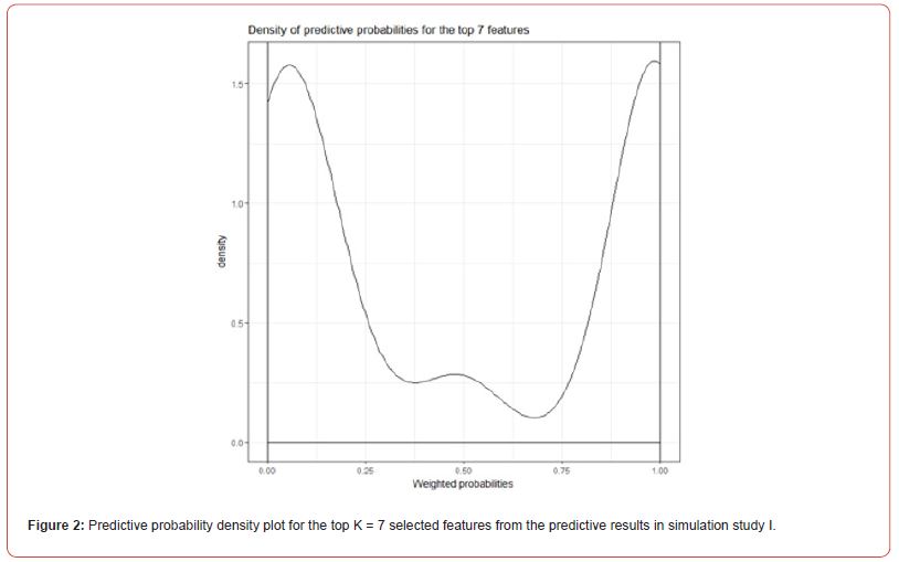
A low-density value at the probability of 0.5 suggests that there was little discordance in the predicted A and B groups for these top seven features. While group classification from weighted probabilities (group A  probability of zero and group B  probability one) provide a level of uncertainty, to further assess the predictive performance of this analyzes, we re-classified each observation with group A being re-defined as those probabilities < 0.5 , and group B re-defined as those observations with probabilities ≥ 0.5 , and compared these predictions with the ground truth. This pooling of information from several features, rather than prediction to each feature (which may vary between features) may provide a more robust alternative approach to identify disease and non-disease groups. We found that this simulation study, our results improved prediction measures with a specificity of one and sensitivity of 0.964 when group prediction was derived from weighted predictive probabilities, highlighting the benefits of this additional analyzes.

Simulation study II

The application of the FSPmix algorithm is intended as an exploratory tool on biological medical data. Alternative applications of the FSPmix include the field of genomics and microarray data, typically where the number of features is often greater than the number of observations. In this instance scalable algorithms are essential in order to broaden their application to both small and large data sets. For this reason, we investigated the performance of the FSPmix algorithm on a large scale set of 1,000 synthetic normalized gene expressions, with hidden disease and non-disease groups. Synthetic data was generated in a similar manner to simulation I as shown in Figure 10 in Appendix A.2. Groups A and B consisted of hundreds of heavily overlapped left (gene.423) and right (gene.161) skewed groups (variance components generated from a uniform distribution), in addition to data generated with the same variance (value of 0.3) but different means (gene 812 for example). As each feature required N = 500 bootstraps, this second simulation study was performed on a High-Performance Computer (HPC) cluster.

Depending on the computational resources available, we found that the computation time taken is greatly reduced when multiple CPUs are allocated to running the FSPmix algorithm. In this instance, it took approximately 1.5 hours to run the FSPmix on 1,000 simulated genes using 10 central processing units (CPUs). It would have taken considerably longer should this simulation study be performed in series (single CPU), nonetheless, in this instance for this simulation study we validated the need to use parallel computing to deliver a scalable algorithm. The FSPmix algorithm identified 737 simulated genes supporting two hidden groups out of a total of 1,000 simulated genes; the FSPmix did not support two groups on 263 genes. Upon investigating the genes which the FSPmix was unable to classify, we found that they had similar densities to a low variance unimodal distribution, where a two component, mixture model would be unsuitable to model such a data set. Figure 3 shows the specificity (blue) and sensitivity (red) for the three different types of simulated genes.

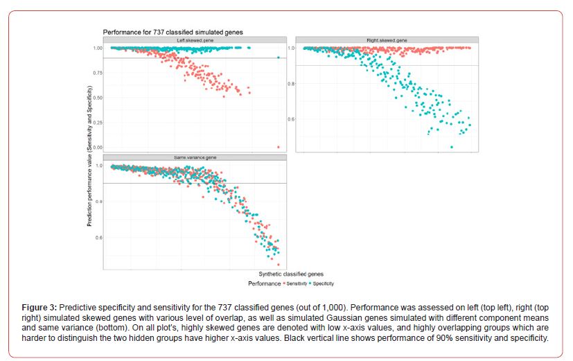
There is a reduction in sensitivity or specificity contingent on which way the simulated data was skewed, whether it was left or right skewed. Regardless of their distribution, the FSPmix showed excellent performance on highly skewed genes with both specificity and sensitivity greater than 0.9. However, as the groups start to merge and become overlapping, simulating a more life-like scenario, there is a drop in performance, which is expected, as a limitation of the FSPmix, is its inability to identify hidden groups on unimodal distributed data. Interestingly we see that on simulated data which was generated by Gaussian distributions with different means but with the same variance (non-skewed data), we see that the performance decreases in a non-linear manner as the two groups increasingly become overlapping, eventually resulting in a long-tailed unimodal distribution (for example gene.325 in Figure 10).

Application to ADNI Case Study

In accordance with Step 1 of Algorithm 1, we first fitted a linear regression to account for variables which could help explain the variation in each set of ROIs. Covariates used in the regression model include gender, diagnosis, age, and apolipoprotein ε 4 carrier and non-carrier status. The residuals of the regression were then retained and those observations for each ROI which supported two groups were classified A, B or C. Amyloid negative participants were those participants with the least amount of global SUVR and high CSF 42 Aβ . In this study data, we expect to see some level of SUVR over all the regions for all participants, however only those participants who are on the AD pathway may have differential amyloid levels in specific ROIs. The FSPmix identified 46 out of 72 ROIs which supported two hidden groups within the data. The remainder of the ROIs did not support two groups suggesting that these features would be poor predictors of amyloid status. Out of the 46 ROIs, our results suggest that the left lingual gyrus was the strongest ROI to distinguish between two groups.

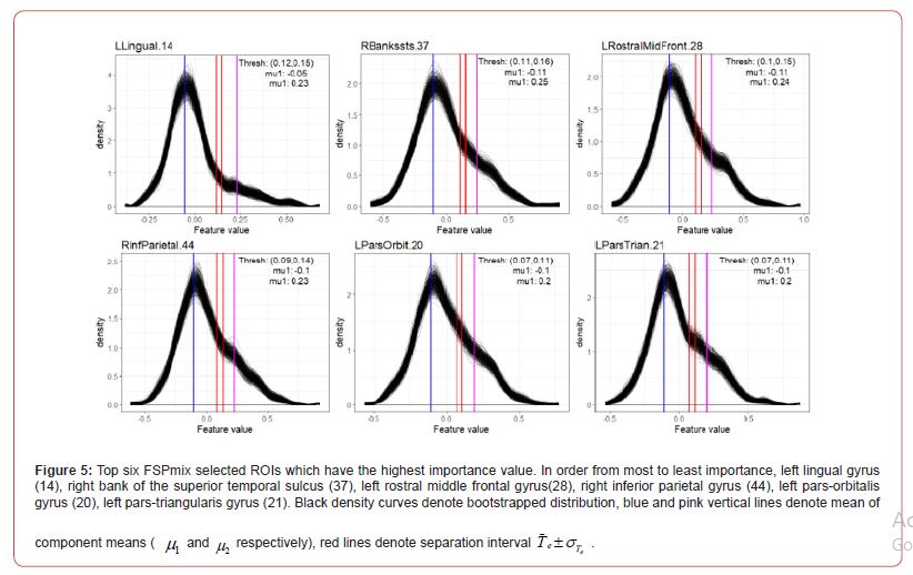
The top left of Figure 5 shows this region has response values skewed to the right, with a large difference in the component means and small separation interval. The other five regions in Figure 5, show the mean of the component means to be closer together and or have slightly larger separation intervals, resulting in smaller _ values. As the majority of the participants in our data are cognitively normal (266 individuals 31%), we suspect that these individuals have low amyloid across all regions resulting in ROI normalized SUVR values to be right skewed, as shown in the bootstrap densities in Figure 11 in Appendix A.2.

Feature Selection and Ranking

To compare the feature selection and importance ranking from FSPmix with other well-known feature selection algorithms, we also applied the case study data to rank ROI features using RFs (features are ranked from high to low mean decrease gini, often shown as the variable importance plot), absolute β ≠ 0 coefficients from the LASSO and the relative influence value from GBM, both ranked from high to low values. As all four algorithms (RF, LASSO, GBM and FSPmix) utilize different approaches to select key features which best describe the response, we expect to see both similarities and differences on the features selected. Similarities in the results may arise due to the strength of each feature which may strongly support differences in the response groups. Differences in feature selection among these algorithms may arise due to the difficulty for each method to define those features that have only a marginal capability to separate response groups, and as such many features will be discarded due to different penalties used. For example, the LASSO is a parametric approach whose results are sensitive to the sparsity value chosen, whereas RF and GBM algorithms rely on an ensemble of decision trees to deduce the key features.

As the scope for this work is to present the FSPmix algorithm, we omit further details on the metrics and inner workings of each competing algorithm and refer the reader to the works by, and for full details on RF, GBM and LASSO algorithms respectively. In this work we used the default settings for the RF and GBM algorithms. Prior to implementing the LASSO, we ran the cross-validation on the generalized linear model via penalized likelihood implementation (cv.glmnet function from the glmnet R package) to determine the optimal sparsity value λ . In this work the choice λ for was chosen to be either the value which returned the minimum mean crossvalidation error or the largest value such that the error is within one standard error of the minimum cross-validation error. Applied to the ADNI data, we found that the λ that returned the minimum mean cross-validation error resulted in 28 features selected by the LASSO. In order to level the playing field for the competing feature selection algorithms, the top 28 features for the RF, GBM and FSPmix were used to create Table 1. Table 1 shows the comparison of these four algorithms and their choice of features which best describe the response for ROIs which received two or more votes. Each feature is assigned one vote if an algorithm selects it as a key indicator based on their respective importance value.

For the sake of this comparison, we disregard how strongly an algorithm prefers specific features, and treat the selected features from different algorithms with the same weight. Features with four votes denotes they were chosen by all four algorithms, and features with two votes denotes that only two algorithms supported this to be an important feature. Analyzes of the 72 ROIs found three features that were selected from all four algorithms to be strongly associated with the response. Taking the union of those features selected from all four algorithms, we saw this number increase to 33 ROIs. The left rostral middle frontal and right middle temporal and precuneus ROIs were selected by all four algorithms to support two hidden disease groups (Table 1). There were 16 ROIs which were selected by three algorithms as important features, with FSPmix supporting ten of those. We note that while the RF and GBM contributed to majority of the votes among all the algorithms (24 and 23 respectively out of 33), both FSPmix and LASSO contributed to 18 votes, suggesting that the FSPmix being an unsupervised algorithm has comparable feature selection capability to alternative supervised algorithms.

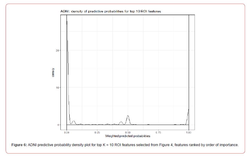
Table 1: Feature selection (33 ADNI ROIs) which best describes non-amyloid accumulators’ binary response comparison between random forest (RF), lasso (L), gbm (G) and FSPmix (F) algorithms. These supported two or more votes from the four feature selection algorithms. FSPmix and LASSO contributed 18 votes listed above, whereas GBM and RF contributed 23 and 24 votes respectively.

Assessment of predictive performance

In order to compare the predictive performance of the 46 features selected by the FSPmix algorithm with another well-known unsupervised classification approach, we investigated the ROI data with a view to predicting amyloid status using k-means clustering with K = 2clusters and compared the specificity and sensitivity with the known response values. The scatter plot in Figure 12 in Appendix A.4 shows the true positive rate (y-axis) compared to the false positive rate (x-axis) for the predicted 46 ROIs. The FSPmix had slightly higher sensitivity and false positive rate in comparison with the predictions from the k-means clustering. The accuracy of both algorithms was computed by the ratio of the sum of all true positives and all true negatives divided by the sum of the total population [27]. The accuracy value ranges from zero denoting extremely poor accuracy to one implying perfect classification. The accuracy from k-means prediction is 0.7099 which is only slightly higher than the prediction accuracy from the FSPmix algorithm of 0.6872. As the FSPmix is intended to be a preliminary exploratory tool to classify feature into binary disease/non-disease groups and search many potentially skewed features, it is reassuring to know that it has comparable prediction accuracy to k-means clustering. However, unlike k-means clustering or other unsupervised classification methods, the FSPmix will also identify and rank key features by order of their importance with respect to the two hidden groups.

Weighted Predictive Probabilities

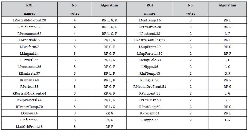
In a similar manner as described in Section 4.1, post classification, prediction, and feature ranking, we computed the weighted predictive probabilities conditional on the top K =10 ROI features. Figure 6 shows the density curves for all the weighted predicted probabilities. It is interesting to note that in this application as the data comprises a large number of nonamyloid pathology (group A) individuals, we see that majority of the probabilities are close to zero. This result also corroborates with the six bootstrap density plots shown in Figure 5, as they are all right skewed suggesting that majority of the group predictions were classed as group A, and hence be assigned a probability value close to zero. As the result in Figure 6 is of the predictive combination of K =10 features (the other four bootstrap FSPmix densities to compliment Figure 5 can be found in Appendix A.4), the few observations which support amyloid pathology groups (predicted as group B) is also evident by the small density curve skewed to the right in Figure 6. The conflicting group predictions among the K =10 features are shown by the small number of observations which were assigned a predictive probability of 0.5.

In this work we propose a scalable unsupervised feature selection and prediction algorithm (FSPmix) and demonstrated its use in an application to the ADNI case study data. Intended as an exploratory method to identify features which support two hidden groups, applied to neuroimaging data, FSPmix identified 46 brain ROIs which strongly supported amyloid pathology and nonpathology groups. Validated on two simulation studies, FSPmix demonstrated high predictive performance on highly skewed synthetic features with a sensitivity and specificity greater than 0.9. As expected in features with overlapping groups, the predictive performance of the FSPmix deteriorates linearly with an inverse relationship for left or right skewed data. Classified features are then ranked by order of importance conditional on the separation of the two hidden groups and further analyzes enables the reclassification of group prediction contingent of user defined top K = 7 selected features, resulting in weighted group prediction probabilities. This re-classification labeling resulted in an increased sensitivity and specificity predicted performance of 0.964 and one respectively.

The second simulation study of 1,000 synthetic genes demonstrated the scalability of the FSPmix algo-rithm, which enabled classification and prediction performance of 737 features. The prediction performance in the large scale, simulation study echoed the results from first simulation study in a linear decrease of sensitivity and specificity as feature group densities became overlapping. Interestingly on simulated gene expression data which had the same variance (different group means and were not skewed) the performance had a non-linear decrease on both sensitivity and specificity. Applied to the ADNI case study data on 72 ROIs of the human brain, the FSPmix identified 46 ROIs which supported amyloid pathology and non-pathology groups. Once ranked, the left lingual gyrus was found to be the single best region in our case study which best discriminates between the two amyloid groups. FSPmix showed similar predictive performance to k-means clustering and identified similar features by order of importance as three commonly used supervised feature selection alternatives. Being a scalable and exploratory tool, a major limitation for the FSPmix algorithm is that it is not suitable for formal statistical inference.

While FSPmix delivers a range of analyzes to aid the user explore classification prediction and feature selection, all the statistical analyzes presented in this work are intended for exploratory purposes only. Future work would be to explore the theoretical statistical properties of the FSPmix methodology, in particular Step 3 of Algorithm 1 which pertains to the bootstrap sampling to enable formal statistical inference for each feature. Another restriction of the FSPmix algorithm is that it is limited to binary classification of each feature. Complex medical diseases often include subgroups of individuals at various stages of pathology, for example in AD the three main broad stages of disease progression are CN to MCI to AD. In this instance FSPmix was applied to generalize the data into two groups, however, this motivates future work to extend the FSPmix methodology and allow for the exploration of user defined subgroups beyond binary disease and non-disease groups. Motivated by the results from our analysis, we propose several extensions to the algorithm.

While the current algorithm is suitable for the exploration of potentially two hidden groups (disease and non-disease) within each feature, future work to extend this to allow the user to search for more than two groups on all or a specific subset of features can easily be accommodated. As this is a parallelized algorithm suitable for large data sets with binary response, application of the algorithm on other large-scale data sets outside the area of AD or medicine in general remains to be investigated. In summary, FSPmix showed comparable predictive and feature selection performance in both simulated and case study applications, demonstrating the potential of this algorithm as a powerful and scalable exploratory tool for both small and large binary data sets.

The authors have declared no conflict of interest.

We wish to thank the Alzheimer’s Disease Neuroimaging Initiative (ADNI) study, including all the clinicians, scientists, participants, and their families. Data collection and sharing for this project was funded by the Alzheimer’s Disease Neuroimaging Initiative (National Institutes of Health Grant U01 AG024904) and DOD ADNI (Department of Defense award number W81XWH-12-2-0012). ADNI is funded by the National Institute on Aging, the National Institute of Biomedical Imaging and Bioengineering, and through generous contributions from the following: AbbVie, Alzheimers Association; Alzheimers Drug Discovery Foundation; Araclon Biotech; BioClinica, Inc; Biogen; Bristol-Myers Squibb Company; CereSpir, Inc; Cogstate; Eisai Inc; Elan Pharmaceuticals, Inc; Eli Lilly and Company; EuroImmun; F. Hoffmann-La Roche Ltd and its affiliated company Genentech, Inc; Fujirebio; GE Healthcare; IXICO Ltd; Janssen Alzheimer Immunotherapy Research & Development, LLC; Johnson & Johnson Pharmaceutical Research & Development LLC; Lumosity; Lundbeck; Merck & Co, Inc; Meso Scale Diagnostics, LLC; NeuroRx Research; Neurotrack Technologies; Novartis Pharmaceuticals Corporation; Pfizer Inc; Piramal Imaging; Servier; Takeda Pharmaceutical Company; and Transition Therapeutics. The Canadian Institutes of Health Research is providing funds to support ADNI clinical sites in Canada. Private sector contributions are facilitated by the Foundation for the National Institutes of Health (www.fnih.org). The grantee organization is the Northern California Institute for Research and Education, and the study is coordinated by the Alzheimers Therapeutic Research Institute at the University of Southern California. ADNI data are disseminated by the Laboratory for Neuro Imaging at the University of Southern California. Funding for this work was provided by the Commonwealth Scientific and Industrial Research Organisation (CSIRO). Computational resources and services used in this work (Simulation study 2) were provided by the High-Performance Computing (HPC) research support, CSIRO.

a) Appendix 1: List of ADNI feature ROIs (Table 2).

b) Appendix 2: Synthetic simulation study data and additional results: Simulated 20 features for FSPmix simulation one study shown in Figure 7. Figure 10 shows randomly selected densities for large scale 1,000 gene synthetic data.

c) Appendix 3: FSPmix ADNI boots trap densities.

d) Appendix 4: ADNI prediction ROC plot.

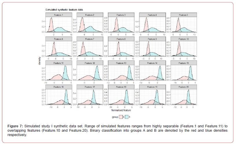
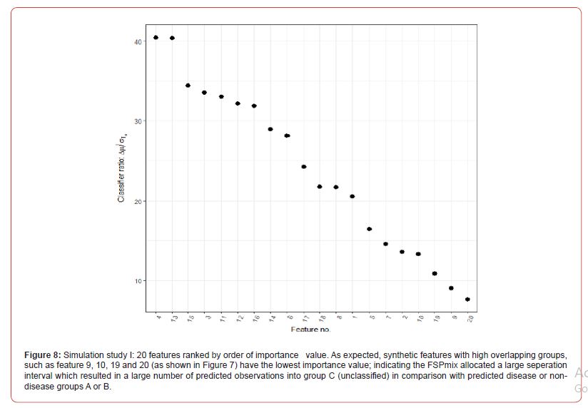
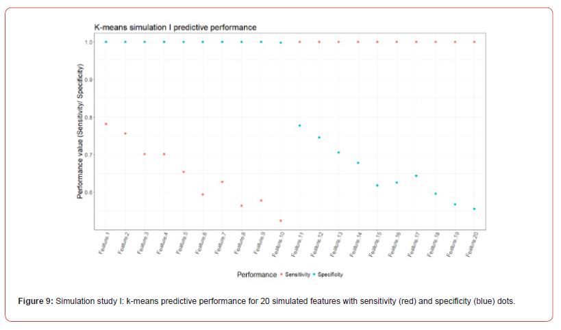
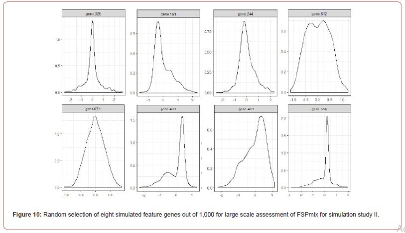
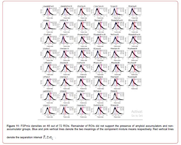
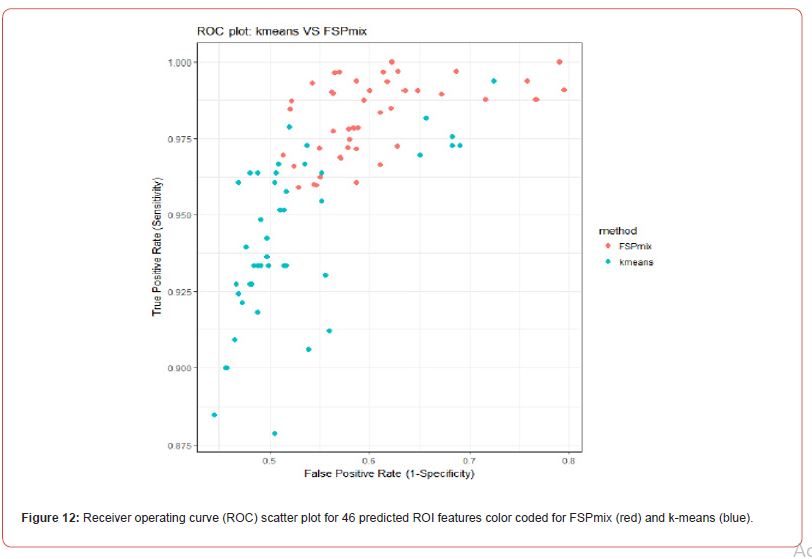
Table 2: Table of 72 PET ROI features from ADNI study listed as per Desikan anatomical atlas. Regions divided into the left (ROI numbers 1-36) and right (ROI numbers 37-72) hemispheres prefaced by ‘L’ and ‘R’ respectively.

1. Kourou K, Exarchos T P, Exarchos K P, Karamouzis M V, Fotiadis D I (2015) Machine learning applications in cancer prognosis and prediction. Comput Struct Biotechnol J 13: 8-17.
2. Cleophas T J, Zwinderman A H, Cleophas-Allers H I (2013) Machine Learning in Medicine. Springer.
3. White N, Johnson H, Silburn P, Mengersen K (2012) Dirichlet process mixture models for unsupervised clustering of symptoms in Parkinson’s disease. Journal of Applied Statistics 39(11): 2363-2377.
4. Breiman L (2001) Random Forests. Machine Learning 45(1): 5-32.
5. Freund Y, Schapire R E (1997) A decision-theoretic generalization of on-line learning and an application to boosting. Journal of Computer and System Sciences 55(1): 119-139.
6. Tibshirani R (2011) Regression shrinkage and selection via the lasso: a retrospective. Journal of the Royal Statistical Society: Series B (Statistical Methodology) 73(3): 273-282.
7. Strobl C, Boulesteix A L, Kneib T, Augustin T, Zeileis A (2008) Conditional variable importance for random forests. BMC Bioinformatics 9(1): 307.
8. Natekin A, Knoll A (2013) Gradient boosting machines, a tutorial. Frontiers in Neurorobotics 7: 21.
9. Palmqvist S, Scholl M, Strandberg O, Mattsson N, Stomrud E, et al. (2017) Earliest accumulation of amyloid occurs within the default-mode network and concurrently affects brain connectivity. Nat Commun 8(1): 1214.
10. Mattsson N, Insel P S, Donohue M, Jagust W, Sperling R, et al. (2015) Predicting reduction of cerebrospinal fluid -amyloid 42 in cognitively healthy controls. JAMA Neurology 72(5): 554-560.
11. Yang T, Wang J, Sun Q, Hibar D P, Jahanshad N, et al. (2015) Detecting genetic risk factors for Alzheimer’s disease in whole genome sequence data via Lasso screening. Proc IEEE Int Symp Biomed Imaging 2015: 985-989.
12. Wu G, Shen D, Sabuncu M (2016) Machine Learning and Medical Imaging. Academic Press.
13. Hartigan J A, Wong M A (1979) Algorithm AS 136: A k-means clustering algorithm. Journal of the Royal Statistical Society 28(1): 100-108.
14. Allen N, Sudlow C, Downey P, Peakman T, Danesh J, et al. (2012) UK Biobank: Current status and what it means for epidemiology. Health Policy and Technology 1(3): 123-126.
15. Weiner M W, Veitch D P, Aisen P S, Beckett L A, Cairns N J, et al. (2013) The Alzheimer’s Disease Neuroimaging Initiative: a review of papers published since its inception. Alzheimer’s & Dementia 9(5): e111-e194.
16. Saeys Y, Inza I, Larranaga P (2007) A review of feature selection techniques in bioinformatics. Bioinformatics 23(19): 2507-2517.
17. Mooney S J, Westreich D J, El-Sayed A M (2015) Epidemiology in the era of big data. Epidemiology 26(3): 390-394.
18. Miller K L, Alfaro-Almagro F, Bangerter N K, Thomas D L, Yacoub E, et al. (2016) Multimodal population brain imaging in the UK Biobank prospective epidemiological study. Nat Neurosci 19(11): 1523-1536.
19. Mueller S G, Weiner M W, Thal L J, Petersen R C, Jack C R, et al. (2005) Ways toward an early diagnosis in Alzheimers disease: the Alzheimers Disease Neuroimaging Initiative (ADNI). Alzheimer’s & Dementia 1(1): 55-66.
20. Weiner M W, Aisen P S, Jack C R, Jagust W J, Trojanowski J Q, et al. (2010) The Alzheimer’s Disease Neuroimaging Initiative: progress report and future plans. Alzheimer’s & Dementia 6(3): 202-211.
21. Shaw L M, Vanderstichele H, Knapik-Czajka M, Clark C M, Aisen P S, et al. (2009) Cerebrospinal fluid biomarker signature in Alzheimer’s Disease Neuroimaging Initiative subjects. Ann Neurol 65(4): 403-413.
22. Mormino E, Kluth J, Madison C, Rabinovici G, Baker S, et al. (2008) Episodic memory loss is related to hippocampal-mediated -amyloid deposition in elderly subjects. Brain 132(5): 1310-1323.
23. Landau S M, Mintun M A, Joshi A D, Koeppe R A, Petersen R C, et al. (2012) Amyloid deposition, hypometabolism, and longitudinal cognitive decline. Ann Neurol 72(4): 578-586.
24. Benaglia T, Chauveau D, Hunter D, Young D (2009) Mixtools: An R package for analyzing finite mixture models. Journal of Statistical Software 32(6): 1-29.
25. Havre Z V, White N, Rousseau J, Mengersen K (2015) Overfitting bayesian mixture models with an unknown number of components. PLOS One 10(7): e0131739.
26. Efron B, Tibshirani R J (1994) An introduction to the bootstrap. CRC press.
27. Taylor J (1997) Introduction to error analysis, the study of uncertainties in physical measurements. University Science Books.