Optimal Weibull Distribution I for Dose-Response Modelling of Theophylline Drug

Dose-response modeling is a crucial tool in various fields, including toxicology, pharmacology, and environmental science, [1] as it enables us to understand how a substance’s dose and its biological response relate to each other. Theophylline, an example of a substance that requires dose-response modeling to maximize therapeutic efficacy and reduce potential toxicity, is a medication that is frequently used to treat respiratory problems. Theophylline is a widely used drug for the treatment of respiratory diseases, such as asthma and Chronic Obstructive Pulmonary Disease (COPD). However, the optimal dosage of theophylline for individual patients remains a challenge due to the complex dose-response relationship. Different models have been proposed to describe theophylline drug data, but dose-response models have suffered a major setback in this regard. Therefore, this study attempted to apply four doseresponse models and evaluate the sensitivity of these models to the theophylline drug data.

The proposed four dose-response models are four parameters loglogistic model, Brain-Cousens hormesis model, Cedergreen-Ritz- Streibig modified log-logistic model, and Weibull distribution I. The four-parameter log-logistic model, which has been widely applied in dose-response analyses, is characterized by its ability to capture various shapes of dose-response curves. This particular model has been used in studies on Paralytic Shellfish Poisoning (PSP) in humans [2] and its application to theophylline dose-response analysis can provide valuable insights into the drug’s efficacy and potential adverse effects. The emergence of the Brain-Cousens hormesis model as a dose-response model has gained attention in recent years. It suggests that low doses of a substance may have a stimulatory effect, while higher doses may lead to inhibitory responses. This model has been applied in different fields, including radiation therapy and environmental science [3]. In the context of theophylline, exploring the potential hormetic effects of the drug can provide valuable information on its dose-dependent benefits and potential risks [4].

Another dose-response model is Cedergreen-Ritz-Streibig’s modified log-logistic model which is a variation of the fourparameter log-logistic model. This was specifically designed to account for non-monotonic dose-response curves. The model has been used in the analysis of Escherichia coli O157 outbreaks, incorporating data from both foodborne and environmental sources [5]. Applying this modified model to theophylline doseresponse modeling can help to understand the drug’s complex biological effects and optimize its therapeutic use. Moreover, Weibull distribution I as a dose-response model is a probability distribution commonly used in survival analysis. It has also been applied in dose-response modeling, as it enables it to estimate other crucial quantities, such as the median Effective Dosage (ED50). In the context of theophylline, the Weibull distribution can provide insights into the drug’s potency and optimal dosage range [6].

Recently, there has been renewed interest in the 4PL model [7]. It was suggested that to completely characterize the functioning of psychopathology items, a four-parameter model is needed. This was later confirmed by the authors [8]. The 4PL model has been found to be effective in computerized adaptive testing as well [9]. The 4PL model’s parameter estimation is a challenging task, [10,11], which is why it has been largely ignored for a long time. However, some recent literature has used a Bayesian approach to estimate item parameters and [12], one interesting work utilizes a mixture model formulation and prior distributions for the parameters [13]. One of the earliest and most well-known dose-response models that allows for hormesis and assesses its significance is the Brain-Cousens model. It has been successfully used in several plant studies. [14- 17], The model has limitations which reduce its robustness and flexibility when applied to real data [18]. Confined to values larger than one, the model can be problematic when fitting curves with inherently low slopes.

Based on the fact that we could not find significant hormesis modelling in 51 dose-response data sets of herbicide toxicity with the Brain and Cousens model. This study aims to comprehensively analyze and compare the efficacy of theophylline drug using doseresponse models to determine the optimal dosage for four doseresponse models. The result of the findings will be used to evaluate the sensitivity of the models and compare the performance of the four models to predicting theophylline drug responses. The rest of the article is arranged as follows; Section one covers the introduction of the study, background of the study and review of related literatures. Section two discussed the research and methods used, method of data collection, method of data analysis, and model specification while section three deals with the analysis of the data. It also contains the results and a discussion of the study. Finally, section four comprises of summary and conclusion.

The analysis of the data was conducted by utilizing R programming language. Secondary data was used for the study and was obtained from Kaggle website at https://www. kaggle.com/datasets/shanmdphd/theophylline The theophylline data frame has 132 rows and 5 columns of data from an experiment on the pharmacokinetics of theophylline. Twelve subjects were given oral doses of theophylline then serum concentrations were measured at 11 time points over the next 25 hours. This data frame contains the following columns:

a) Subject: a factor identifying the subject.

b) Wt: Weight of the subject (kg).

c) Dose: Dose administered to the subject (mg/kg).

d) Time: Time since drug administration when the sample was drawn (hours).

e) Conc: Theophylline concentration in the sample (mg/L).

Dose-Response Model

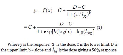
Considering a set of n dose-response curves and assuming that, apart from a parameter vector that might vary depending on the curve, each dose-response curve’s reaction follows a nonlinear curve given by the function f. Therefore, the mathematical expression relating to the dose-response curve is obtained as (1)

Models

The four models for sigmoidal dose-response curves widely employed in this study to fit the most suitable model for the data are explained as follows.

The Four-Parameter Logistic Function is given as (2)

Where b denotes the relative slope around e, c is the lower limit, d is the upper limit and e also denoted 50% effective dose (ED50) explained vividly the interpretation of the parameters to (2). The model showed that the logistic function is symmetric around e with two slightly different parameterizations, one where ED50 is a model parameter, that is e in (2), and another where the logarithm of ED50 denoted by  e , is a model parameter as in (3)

Brain-Cousens Hormesis Model

Brain-Cousens modified log-logistic models for describing u-shaped hormesis are given as (4)

Where b denotes the relative slope around e, c is the lower limit, d is the upper limit, e denoted 50% effective dose (ED50) and f is the size of the hormesis effect. The larger the value, the larger the hormesis effect. f = 0 corresponds to no hormesis effect, and the resulting model is the four-parameter log-logistic model. This parameter should be positive for the model to make sense.

Cedergreen-Ritz-Streibig Modified Log-Logistic Model

The Cedergreen-Ritz-Streibig modified log-logistic model for describing (inverse u-shaped or j-shaped) hormesis is given as (5)

Where b denotes the relative slope around e, c is the lower limit, d is the upper limit, e also denoted 50% effective dose (ED50), f is the size of the hormesis effect and α is the scale parameter, also called the characteristic life parameter.

Weibull Distribution I

The Weibull distribution I is a continuous probability distribution. It models a broad range of random variables, largely like a time to failure or time between events. The Weibull distribution I is given by the expression (6)

Where γ is the shape parameter, also called the Weibull slope or the threshold parameter, α is the scale parameter, also called the characteristic life parameter and μ is the location parameter, also called the waiting time parameter or sometimes the shift parameter.

The standard Weibull distribution is derived, when μ = 0 and α =1, then, (6) reduced to (7)

Table 1: Model functions and corresponding name of some of the most important built-in models available in drc.

The parameters c and d denote the horizontal asymptotes or limits, whereas the parameter b is the relative slope at the inflection point of the resulting dose–response curve. The parameter e corresponds to the dose where the inflection point is located. The original, untransformed dose is denoted x throughout.

The analysis was carried out using the R programming language. The variables of data for the analysis are drug dose (in mg/kg) and concentration (mg/L). Figure 1 shows the scatter plot; the study has a discrete view of what the drug response is. However, we need a continuous representation of the drug-response relationship, so we can obtain a full view of the response caused by the drug at any given concentration. To obtain this continuous view, we need to use a ‘curve fitting’ algorithm. A curve fitting algorithm optimizes the parameters of a curve or function so that it ‘adjusts’ or ‘fits’ to the data as closely as possible. With the adjusted curve, we will be able to interpolate and extrapolate response values, hence we will know the response at any given drug concentration. Table 2 presented the analysis of the four models considered namely, four-parameter log-logistic model, Brain-Cousens hormesis model, Cedergreen- Ritz-Streibig modified log-logistic model, and Weibull distribution I (Figure 2). Figure 3 did not show any significant variation when we considered the log scale of the data.

Table 2: Estimate the optimal parameters.

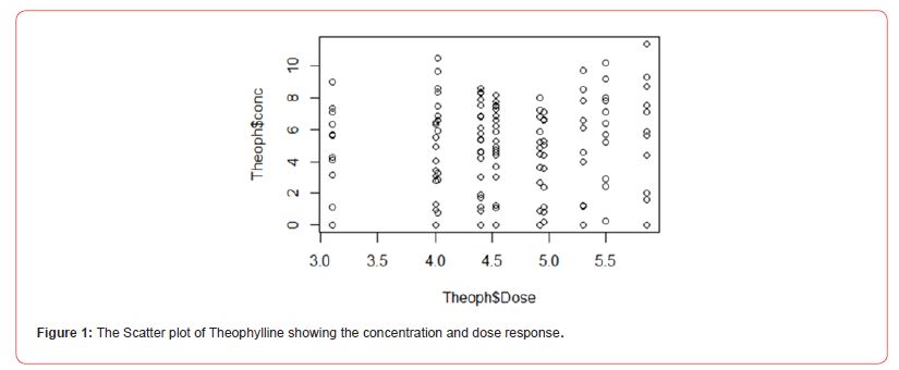
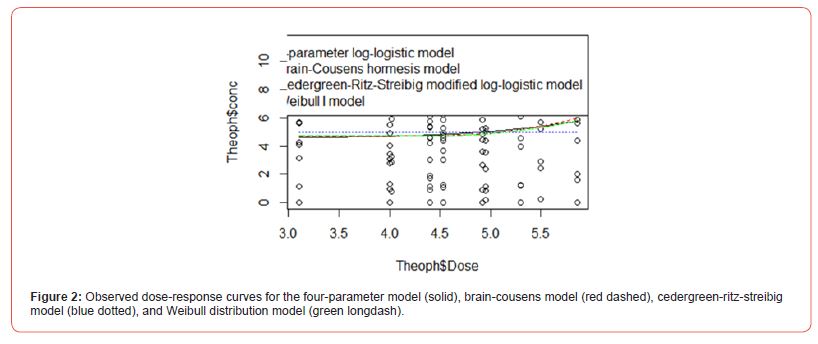
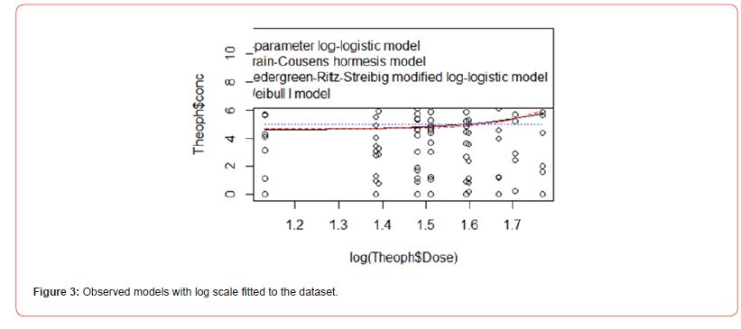
Table 3 revealed that Weibull distribution 1 outperformed other models with the least BIC value of (294.4214). Therefore, Weibull distribution 1 is the best model for modelling theophylline drug. Figure 4 shows the sensitivity change in the response when the parameter value is perturbed by a small value. Parameter D has the highest sensitivity, so it will have the highest influence on the response. Parameter D has the highest sensitivity at low doses, so it will be important to have enough samples at low doses. BIC lower is for Weibull I model. In the graph, we can see that the Cedergreen- Ritz-Streibig Modified Log-Logistic Model and the Brain-Cousens hormesis model give very similar fits though the Weibull I model was added to ascertain the best model fit which shows a sharp decline at a high dose. Weibull, I model shows significant variation of the model fit. When given the choice between a simpler model and a more complex model which gives almost the same fitted values, we choose the simpler model. Therefore, Weibull I model is more sensitive to model Theophylline drug data.

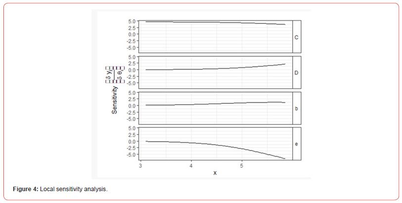
Table 3: The model fits based on BIC value.

Summary

Theophylline is a medication that is used to treat asthma and chronic obstructive pulmonary disease (COPD) by relaxing the muscles of the airways. It is a bronchodilator, which means it opens up the airways in the lungs, making it easier to breathe and preventing wheezing and shortness of breath. There are four different models that can be used to describe the dose-response relationship of theophylline. This study compared four Doseresponse models namely, four parameters log-logistic model, Brain-Cousens hormesis model, Cedergreen-Ritz-Streibig modified log-logistic model, and Weibull distribution I to predict the best model for theophylline dosage and its corresponding physiological properties through sensitivity analysis and Bayesian information criteria (BIC). The findings revealed that Weibull distribution 1 outperformed other models based on BIC model comparison with the least BIC value of 294.4214. Therefore, Weibull distribution 1 is the best model for modelling theophylline drug. Also, a sensitivity analysis was carried out that shows the robustness of the model. Weibull, I model shows a significant variation of the model fit with a sharp decline at high dose. Therefore, Weibull I model is more sensitive to model Theophylline drug data.

Conclusion

In this study, four models were evaluated to fit the doseresponse data for theophylline. All four models provided a good fit, but the Weibull distribution 1 was found to be the best one to describe the data. This is because it is the only model that can accurately capture the hormetic effect of theophylline.

Availability of Data and Materials: Data sharing is not applicable to this article as no datasets were generated during the current study. The data used was obtained from Kaggle website with link https://www.kaggle.com/datasets/shanmdphd/theophylline

The author(s) received no funding for this study.

The author declares that he has no competing interests.

This manuscript was conceptualized and written by Kupolusi J.A. while Akindolani Toluwalope did the data analysis, interpretation and reporting. Therefore, the authors contributed significantly to the write-up.

None.

1. Agathokleous E, Calabrese EJ (2019) Hormesis: The dose response for the 21^st century: The future has arrived. Toxicology 425: 152249.
2. Arnich N, Thébault A (2018) Dose-Response Modelling of Paralytic Shellfish Poisoning (PSP) in Humans. Toxins 10(4): 141.
3. Duncan F, Kimler B, Briley S (2016) Combating radiation therapy-induced damage to the ovarian environment. Future Oncology 12(14): 1687-1690.
4. Calabrese E J (2008) Hormesis and medicine. Br J Clin Pharmacology 66(5): 594-617.
5. Strachana J, Michael P, Fumiko K, Rotariu O, Ogden LD (2005) Dose response modelling of Escherichia coli O157 incorporating data from foodborne and environmental outbreaks. Int J Food Microbiology 103(1): 35-47.
6. Mould DR, Walz AC, Lave T, Gibbs JP, Frame B (2015) Developing Exposure/Response Models for Anticancer. CPT: Pharmacometrics Syst Pharmacol 4(1): 12-27.
7. Reise SP, Waller NG (2003) How many IRT parameters does it take to model psychopathology items? Psychol Methods 8(2): 164-184.
8. Waller NG, Reise SP (2010) Measuring psychopathology with nonstandard item response theory models: Fitting the four-parameter model to the Minnesota Multiphasic Personality Inventory. American Psychological Association pp. 147-173.
9. Rulison KL, Loken E (2009) I’ve Fallen, and I Can’t Get Up: Can High-Ability Students Recover from Early. Appl Psychol Meas 33(2): 83-101.
10. Loken E, Rulison KL (2010) Estimation of a four-parameter item response theory model. Br J Math Stat Psychol 63(3): 509-525.
11. Culpepper SA (2016) Revisiting the 4-parameter item response model: Bayesian estimation and application. Psychometrika 81(4): 1142-1163.
12. Waller NG, Feuerstahler L (2017) Bayesian Modal Estimation of the Four-Parameter Item Response Model in Real, Realistic, and Idealized Data Sets. Multivariate Behav Res 52(3): 350-370.
13. Meng X, Xu G, Zhang J, Tao J (2020) Marginalized maximum a posteriori estimation for the four‐parameter logistic model under a mixture modelling framework. Br J Math Stat Psychol 73(1): 51-82.
14. Schabenberger O, Birch JB (2001) Statistical Dose-Response Models with Hormetic Effects. Human and Ecological Risk Assessment 7(4): 891-908.
15. Schabenberger O, Tharp BE, Kells JJ, Penner D (1999) Statistical tests for hormesis and effective dosages in herbicide dose response. Agronomy Journal 91(4): 713-721.
16. Belz RG, Cedergreen N, Sørensen H (2008) Hormesis in mixtures Can it be predicted? Sci Tottal Environ 404(1): 77-87.
17. Belz RG, Cedergreen N (2010) Environmental and Experimental Botany 69(3): 293-301.
18. Cedergreen N, Ritz C, Streibig JC (2005) Improved empirical models describing hormesis. Environ Toxicol Chem 24(12): 3166-3172.