


 Review Article
Decomposition of Moran’s Coefficient to Detect Non- Multicollinear, Non-Zero, Eigen-Autocorrelated, Non-Gaussian Coefficients in Colorectal Cancer Estimator Determinants Epidemiologically Sampled in Hillsborough County, Florida
Received Date: February 04, 2026; Published Date: February 17, 2026
Abstract
Despite the production of state-level Colorectal Cancer (CRC) incidence statistics, there are currently no precision count variable models to
understand localized incidence rates of CRC. This article aims to utilize a predictive county variable model with semi-parametric eigen spatial
autocorrelation to map Hillsborough County-level CRC incidence rates using zip code census data. The first is an over-dispersed Poisson
regression model that uses a negative binomial model with a non-homogeneously distributed mean to account for outliers. An eigenfunction, eigen
decomposition, and spatial filter technique is presented. The dependent variable was the incidence percentage of CRC at the county level, while
independent variables included sociodemographic indicators obtained from the U.S. Census Bureau. This study used sociodemographic information
at the zip code level in Hillsborough County, Florida, to investigate the geographical aggregation of colorectal cancer cases.
Only the white population emerged as a significant predictor in the Poisson regression model, which demonstrated a non-dispersed paradigm.
Several non-zero autocorrelated clusters were found across different zip codes in Hillsborough County using a second-order eigenfunction eigen
decomposition. A spatial autocorrelation hot and cold spot analysis was conducted. This analysis identified zip codes with the highest and lowest
predicted likelihood of CRC incidence. The identified zip code locations were 33578, 33511, and 33647 in southern Hillsborough County in the
Brandon and Riverview area. The suggested method found hotspots for colorectal cancer where the white population is the main risk factor, which
led to greater hotspot concentrations in Brandon and Riverview. Future studies should encourage routine colorectal cancer screening among
individuals in these at-risk locations and investigate the method’s applicability at the state level.
Keywords:Colorectal cancer; Screening; Poisson; Spatial autocorrelation; Food insecurity; primary care; Hillsborough county
Introduction
Colorectal cancer (CRC) is a type of cancer found within the large intestine, also known as the colon, and the rectum, which is the last segment of the colon connecting to the anus. Polyps, or abnormal pockets of cellular growth, can form along the large intestinal walls and rectum, but these polyps can be removed from the colon while they are still benign. If these polyps are not removed in a timely manner, they can become cancerous, leading to rapid cell growth in other regions of the colon with the possibility of the cancer metastasizing (Moffitt Cancer Center, n.d.). Clinical presentations and symptoms can include rectal bleeding, blood in the stool, chronic constipation, diarrhoea, and changes in the frequency of one’s bowel movements (Moffitt Cancer Center, n.d.). The presence of these symptoms indicates that treatments such as a diagnostic colonoscopy, complete blood count panels, tumor marking tests, and biopsies need to be utilized (Moffitt Cancer Center, n.d.). Colorectal Cancer is diagnosed on a spectrum of stages from 0-4, with increasing complexities associated with each one.
Stage 0 refers to cancer cells being found in the lining of the colon that have not yet spread to surrounding lymph nodes, Stage 1 to cancer cells being found in the lining and connective tissues beneath the colon’s mucous membrane, and Stage 2 to the cancer cells spreading beyond the colon lining into the muscles lining the abdomen. Stage 3 indicates the aggressive spread of the cancer to surrounding organs and lymph nodes, while Stage 4 indicates the distant spread to the lungs or liver [1]. When the cancer is diagnosed at any one of these stages, a combination of chemotherapy, surgery, and radiation therapy can be utilized to put the cancer into remission. Despite a plethora of emerging research and treatment methods of CRC, it is the third most commonly diagnosed cancer in the United States and the third leading cause of cancerous deaths [2]. Because this cancer often develops before the onset of symptoms, there are several routine screening methods used to detect cancerous polyps and to prevent their rapid progression.
The established screening recommendations for primary care physicians from the U.S. Preventive Services Task Force (USPSTF) are to provide Fecal Occult Blood Testing (FOBT) every year and regular colonoscopies to patients 45 years and older, except starting earlier for at-risk patients [2]. Although screening protocols have proven to be effective in early diagnosis in those with access, there are still significant discrepancies in accessibility and death toll. Unfortunately, over 30% of adults aged 50–75 years have not been screened for CRC according to national guidelines, which contributes to the cancer’s high morbidity and mortality rates [3]. Due to statistical discrepancies and rising death toll among specific ages and ethnicities, this warrants a deeper investigation into health outcomes related to the social determinants of health. Literature suggests that a culmination of local social determinants of health plays a significant role in preventative screening accessibility, especially regarding race, ethnicity, socioeconomic status, education level, health literacy, and health insurance status [4].
Preventive screening is vital in the early diagnosis and early surgical interventions that are used to put colorectal cancer into remission. A lack of screenings can lead to increased cancer severity, the use of highly aggressive surgical and chemotherapy treatments, metastatic complications due to unchecked cell growth, and overall increased mortality [5]. Although Hillsborough County statistics suggest an overall 43.9% incidence of CRC, non- Hispanic black Americans display the greatest incidence and mortality of this largely preventable disease, which indicates a presence of multifactorial societal shortcoming, especially access to preventative and diagnostic screenings [6]. More specifically, data from the Surveillance, Epidemiology, and End Results (SEER) program reveal that Black Americans’ overall incidence of CRC is 41.9 per 100,000, as compared to that of White Americans of 37.0 per 100,000, which further indicates a persistent weakness in the preventive care of Black Americans [7].
In addition, Native Americans are second to Black Americans in mortality at 14.0 per 100,000, as compared to White Americans at 12.9 per 100,000, which indicates other ethnicities’ shortcomings in the prevention of CRC [7]. Because the Hillsborough County incidence statistic of 43.9% does not consider racial, ethnic, and regional variations, the downstream statistics at the state, county, and zip code level will reveal greater implications of the social determinants of health on the incidence of CRC, especially regarding race, socioeconomic status, and insurance accessibility [8]. This study aims to identify leading barriers in preventative screenings for CRC and provides greater implications to create targeted, local screening initiatives at the zip code level in Hillsborough County. Spatial cluster detection is an important tool in Colorectal Cancer [CRC] cancer surveillance to identify areas of elevated risk and to generate subsequent hypotheses about the etiology [9].
Establishing precise county, zip code geolocation of an epidemiological, stratified, CRC geospatial cluster may predict the future trend of the cancer locally and inform control strategies. A spatial disease cluster is definable as an area with an unusually higher disease incidence rate National Cancer Institute: Cancer Clusters, but the term has been vaguely employed in the literature to refer to a population-based, cancer stratified, geographic location [henceforth geolocation] due to the complex interaction between multiple epidemiological co-factors believed to contribute to such an event [10]. County, zip code, colorectal cancer [CRC] cluster identification is heavily dependent on the accuracy of the methodological design employed to estimate the local relative risk as compared to the control [11]. A prognosticative geospatial cluster analysis of CRC incidence rates may also provide knowledge on the relationships between risk factors and county, zip code, and potential endemic geolocations.
This would enable policymakers to develop tailored interventions in areas where the CRC risk is greater. By statistically identifying and regression mapping available online racial, sociodemographic, and socioeconomic census data, evidence on county, zip code, clustering patterns of CRC incidence, specifically related to the geospatial aggregation /non-aggregation-oriented [i.e., hot and cold spot] geolocations and their respective estimator determinants may be determinable and prioritizable. In exploring mathematical hypotheses for leukaemia, Satardekar et. al. (2024) [12] proposed using a second-order eigenfunction eigen decomposition for determining hot and cold spots of clusters of leukaemia stratified by racial, sociodemographic, and Land Use Land Cover [LULC] determinants. This was the first contribution in oncological modelling literature that an eigen-spatial filter eigenfunction algorithm was employed for predictive hot and cold spot modelling at the county and zip code level. Firstly, in Satardekar et al. (2024) [12], an over-dispersed Poisson count variable leukaemia regression model was constructed to generate a parameter hierarchy.
Thereafter, an eigenfunction, eigen-spatial filter algorithm identified potential, hyper/hypo-endemic, aggregation/nonaggregation- oriented leukaemia clusters. The second-order eigenfunction eigen decomposition revealed multiple non-zero autocorrelated clusters throughout various zip codes in Hillsborough County. The hot spots were in 33647, 33578, and 33511, and the cold spots were in 33621, 33503, and 33530. The model identified leukaemia hotspot determinants as Whites and Asians aged 65+. Urban residential communities in 33647 were most vulnerable to leukaemia. The most common landscape variable associated with leukaemia was urban residential. Geospatial eigenfunction eigen-decomposition uncertainty-oriented treatment may be applicable to an empirical dataset of county zip code, racial, sociodemographic, and socioeconomic estimator determinants to improve understanding of a range of CRC-related issues, including the mechanisms driving local hyper/hypo-endemic, hot and cold spot, stratified, and potential determinants.
An oncologist or researcher in practice, could essentially interpret eigen-spatial autocorrelation in a CRC county, zip code hot and cold spot, prognosticative epidemiological model in multiple different ways: self-correlation, map pattern, a diagnostic tool, a missing variables surrogate, a spatial process mechanism, a spatial spill over effect, an outcome of areal unit demarcation (re. the MAUP), redundant information, and a nuisance parameter. These statistical methods can be combined with environmental factors exposure to understand county zip code epidemiological drivers of local CRC; however, such studies remain limited for CRC in highincidence areas due to erroneous forecasting of aggregation/nonaggregation, oriented, potential, hyper/hypo-endemic estimator determinants [13]. Regrettably, statistics currently utilized in CRC research are content with the traditional linear regression to examine determinant non-independence (i.e., multicollinearity), zero-inflated non-homoscedasticity (i.e., uncommon error variance), non-Gaussian zero autocorrelation (i.e., geographic chaos), and other violations of regression assumptions in space and geography.
Linear regression cannot denoise spatial error in models due to violations of regression assumptions in space and geography [14]. The decomposition of Moran’s coefficient into uncorrelated, eigen-orthogonal map pattern components may reveal global heterogeneities necessary to capture noisy, stochastic, latent chaotic spatial biasness [e.g., skewed, zero, eigen-autocorrelated heteroscedastic multicollinear coefficients] embedded inconspicuously in regressively prognosticated, stratifiable CRC county, zip code epidemiological model forecast determinants. Moran’s I is a measure of spatial autocorrelation [15]. Spatial autocorrelation is characterized by a correlation in a signal among nearby locations in space. Spatial autocorrelation is more complex than 1 one-dimensional autocorrelation because spatial correlation is multi-dimensional (i.e., 2 or 3 dimensions of space) and multi-directional [14]. Moran’s index is an important statistical measure used to quantify the presence or absence of residual, zero/non-zero, eigen-spatial autocorrelation, thereby determining the selection orientation of spatial statistical uncertainty-oriented algorithmic denoising methods.
Moran’s index is chiefly a statistical measurement rather than a mathematical model [15]. In this experiment, we employed the Spatial Autocorrelation Moran’s I tool in ArcGIS ProTM to measure residual, zero autocorrelation [i.e., geographic chaos] in an empirical, eigen-decomposed, CRC-related, zip code dataset of sociodemographic and socioeconomic determinants in Hillsborough County. Using the set of stratified, geosampled capture points, diagnostic, feature attributes of the covariates, this tool evaluated whether eigenvectors derived from a weighted, aggregation/non-aggregation-oriented, CRC-related hyper/hypoendemic model were clustered, dispersed, or random at the county zip code level. We assumed the tool could calculate the Moran’s I value and both a z-score (i.e., standard deviations) and a p-value to evaluate the significance of the eigen-orthogonalized, diagnostic, zip code-stratified, CRC determinants. Our assumption was that a second-order eigenfunction eigen decomposition would reveal multiple non-zero autocorrelated geospatial clusters throughout various zip codes in Hillsborough County.
There has been increasing interest in the analysis of geographically distributed, diagnostically stratifiable CRC data, motivated by a wide range of research problems, such as the inability to quantify violations of regression assumptions in space and geography in causative, hyper/hypo-endemic, regressable covariates of county, zip code stratifiable, hot and cold spot epidemiological geolocations. Traditionally, two types of correlations are involved in epidemiological, CRC-related, regression, estimator determinant models: the correlation between multiple outcomes at one hot or cold spot geosampled, capture point geolocation, and the spatial correlation between the geolocations for one particular outcome. Unfortunately, county or district-level, aggregation/non-aggregation-oriented, zip code stratified, estimator determinant, prognosticative, epidemiological CRC regression models contributed to the literature only consider one type of correlation while ignoring or inappropriately modeling spatial count data with dichotomous [i.e., logistic] probabilities.
The main problem with logistic binary probabilities for optimally regressively quantifying county or district-level CRC forecast regression models is that the probability of the positive outcome is bounded between 0 and 1. This means that while stratifiable, county, CRC, prognosticative, epidemiological modelled determinants can provide insights into the likelihood of a geospatially regressively detected zip code, hot or cold spot, they cannot predict the exact number of occurrences. One of the key challenges in logistic regression is the interpretation of the odds ratio, which compares the probability of success to the probability of failure [16]. Odds ratios greater than 1 indicate a higher likelihood of the event occurring, while those less than 1 suggest a lower likelihood. However, this interpretation is not straightforward, as it would not directly translate to numerical discrete integer values in a county or zip code, stratifiable, hot or cold spot, empirical, geosampled, explanatory, estimator, determinant CRC dataset. Another challenge in binary logistic probabilities is the handling of outlier data, which can skew the results of the regression model and estimator determinants.
Unlike linear regression, logistic regression does not assume a linear [i.e., non-spatial] relationship between the dependent and independent variables, making it non-robust for quantification of linear relationships in an epidemiological forecast-oriented, county, zip code, aggregation/non-aggregation-oriented CRC model. Furthermore, it can be computationally expensive to fit stratified, diagnostically stratifiable, county, CRC-related, capture point vulnerability models with multiple, zip code stratifiable, hot and cold spot, cluster causation, explanatory, estimator determinants, which can be a limitation in certain prognosticative regression modelling scenarios. Unfortunately, currently, nonlinear CRC and epidemiological regression models contributed to the literature are not robust to stochastic randomness of errors. Stochastic error (or random error) is the variability in measurements that cannot be predicted or eliminated [14]. It is inherent in any measurement process in the CRC forecast regression model. The evidence comes from cohort studies in categorical, linear, and nonlinear dose– response meta-analyses.
For example, Dagfinn et al. (2011) [17] included 19 prospective studies that reported relative risk estimates and 95% confidence intervals (CIs) of CRC associated with fruit and vegetable intake. Random effects models were used to estimate summary relative risks. The summary relative risk for the highest vs the lowest intake was 0.92 (95% CI: 0.86–0.99) for fruit and vegetables combined, 0.90 (95% CI: 0.83–0.98) for fruit, and 0.91 (95% CI: 0.86–0.96) for vegetables (P for heterogeneity= .24, .05, and .54, respectively). The inverse associations appeared to be restricted to colon cancer. In linear dose–response analysis, only intake of vegetables was significantly associated with colorectal cancer risk (summary relative risk = 0.98; 95% CI: 0.97–0.99), per 100 g/d. However, significant inverse associations emerged in nonlinear models for fruits (nonlinearity < .001) and vegetables (nonlinearity = .001). The greatest risk reduction was observed when intake increased from very low levels of intake. Based on a meta-analysis of prospective studies, there is a week but statistically significant nonlinear inverse association between fruit and vegetable intake and colorectal cancer risk.
There was no evidence of uncertainty residual testing of the heterogeneity of the model forecasts; hence, there was no evidence of small-study bias in the estimated determinants. Although nonlinear least squares estimation models (Exponential, Gompertz, Verhulst, and Weibull) have been computed for quantifying errors in some epidemiological, CRC, and county regression models contributed to the literature, the estimates from these paradigms have not been able to improve the probability modeling of stratified epidemiological vulnerability hot and cold model forecasts using these methods at the zip code level. Our objectives in this experiment were to generate a residual eigenautocorrelation map and to conduct a non-Gaussian uncertaintyoriented test to quantitate violations of regression assumptions in space and geography for precisely statistically delineating zip code, stratifiable, hot, and cold geolocations and their respective estimator determinants. In so doing, we assumed we would be able to implement a social messaging platform targeting potential CRC patients in Hillsborough County, Florida, USA.
Methodology
To alleviate stratified CRC uncertainty estimator determinant hot and cold spot, non-Gaussian noise due to violations of regression assumption in space and geography at the county, zip code level, we adopted a hierarchical, generalizable, nonfrequentist, uncertainty-oriented, prognosticative model approach. We residually investigate zero autocorrelation, heteroscedasticity, and multicollinearity in an empirical dataset of multivariate, geosampled, county, georeferenced, stratified, racial, sociodemographic, and socioeconomic, epidemiological estimator determinants geosampled in Hillsborough County at the zip code level. Our assumption was that by denoising multiple types of uncertainty-oriented, non-Gaussian, deviant distribution trajectories, we would be able to capture unobserved heterogeneity in the regressed aggregation/non-aggregation-oriented, potential hyper/hypo-endemic, CRC prognosticative, county zip code, estimator determinant models dissimilar to those presented in the literature. Our research hypothesis was that a second-order eigenfunction eigen decomposition and a non-frequentistic semiparametric, prognosticative, regression, uncertainty-oriented model can elucidate county-level, CRC vulnerable zip code populations by prioritizing stratifiable, racial sociodemographic and socioeconomic covariate heterogeneity in an empirical dataset of census stratified estimator determinants to identify the spatial distribution of high-risk populations in Hillsborough County.
Population and Sample
Part of the Tampa–St. Petersburg–Clearwater Metropolitan Statistical Area, Hillsborough County, is situated in the west-central region of the U.S. state of Florida. With 1,459,762 residents, this county is among the most populous in the state, according to the U.S. Census Bureau. With an annual growth rate of 3.7%, the population of Hillsborough County was expected to be 1,513,301 in 2022 (United States Census Bureau, 2020) [18]. The county’s total area is 1,266 square miles (3,279 km2), of which 246 square miles (637 km2) (19.4%) are covered by water and 1,020 square miles (2,647 km2) are land (Florida Water Atlas, 2025) [19]. Several significant bodies of water, including the Little Manatee River, the Hillsborough River, and the Alafia River, are located in Hillsborough (Florida Water Atlas, 2025) [19]. Over 84% of the county’s total land area, or about 888 square miles (2,300 km2), is unincorporated. 163 square miles (420 km2) are made up of municipalities. The county is located halfway along Florida’s west coast, according to its current borders. There are 55 standard zip codes in Hillsborough County, as seen in Figure 1 (Hillsborough County Florida ZIP Codes - Map and Full List, 2025) [20]. The American Community Survey (ACS) U.S. Census data from 2020 was used to collect zip code-level data for this study (United States Census Bureau, 2020) [18]. The countylevel incidence of CRC was obtained from Florida Health Charts. (www.flhealthcharts.gov, n.d.).

Study Variables
Table 1: Global Moran’s I Diagnostic Summary of Georeferenced Zip Code Stratified Hot/Cold Spot Autocorrelated County Level CRC Incidence.

This study constructed zip code probabilities from populationstratified CRC cases related to socioeconomic status, age, education level, insurance status, and racial-related covariates (Table 1), which were acquired from the U.S. Census Bureau (2020) [18]. To obtain the dependent variable that was regressed against with the covariates throughout this study, a population stratification was completed per zip code. To calculate these values, the incidence of CRC in Hillsborough County, 43.9%, was set equal to the estimated population of Hillsborough County, 1,580,000. Each zip code population was then set equal to an unknown variable X. To acquire X, the following equation was used for each zip code: X=(43.9 * Zip Code Population)/ 1,580,000. This allowed for a predictive CRC incidence value to be found for each zip code in our area of study. Our covariates are centered around sociodemographic details: age 45+, race, education, and insurance status.
Study Instruments
We calculated Moran’s I Scatterplot in PySal. We standardized the sampled estimator determinants as z = (x −mean( x)) / std ( x) . This rendered the standardized value of x for each zip code in Hillsborough County. We subsequently calculated the spatial lag. This was done by determining the average of neigh boring values for each zip code region, weighted by spatially sampled CRC racial, sociodemographic, and socioeconomic stratified weights. w_ z =W * z where: W was the spatial weight matrix (e.g., queen or rook contiguity). * Denoted matrix multiplication. and w_ z was the spatial lag of the standardized CRC stratified determinants. We plotted the scatterplot X-axis. and the Y-axis. We added a regression line. The slope of this line was Moran’s I.
The Moran’s I statistic for quantitating zero/non-zero eigenspatial
autocorrelation was , where Z1 was the deviation
of a racial, sociodemographic or socioeconomic stratified, CRC,
county, zip code for feature I from its mean ( x1 − X0) , wij is
the weight quantitated between i an j where n is equal to the
number of determinant features and S0 is the aggregate of all the
spatial weights
where Z1 was the deviation
of a racial, sociodemographic or socioeconomic stratified, CRC,
county, zip code for feature I from its mean ( x1 − X0) , wij is
the weight quantitated between i an j where n is equal to the
number of determinant features and S0 is the aggregate of all the
spatial weights 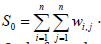 .
.
The Python Code for calculating Moran’s I in PySAL was:
import geopandas as gpd
import libpysal
from esda.moran import Moran
from splot.esda import moran_scatterplot
gdf = gpd.read_file(“your_shapefile.shp”)
x = gdf[‘your_variable’].values
# Create spatial weights
w = libpysal.weights.Queen.from_dataframe(gdf)
w.transform = ‘r’
# Calculate Moran’s I
mi = Moran(x, w)
# Plot scatterplot
moran_scatterplot(mi)
Data analysis
A spatial autoregressive model [SAR] model specification was subsequently constructed to describe the autoregressive variance, non-Gaussian. zero autocorrelated, non-multicollinear, heteroscedastic, potentially asymptotically biased, aggregation/ non-aggregation-oriented determinants. For non-time seriesdependent forecast modeling estimator determinants, the SAR model furnishes an alternative specification [14]. Here, the SAR model was written in terms of matrix W The resulting SAR model specification took on the following form:

where μ was the scalar conditional mean of Y , and ε was an n-by-1 error vector whose elements were statistically independent and identically distributed (i.i.d.) normally random variates. The spatial covariance matrix for equation (2.4), fit the diagnostic, CRC eigen-decomposed i.d.d. covariates using

where E (•) denoted the calculus of expectations, I was the n-by-n identity matrix denoting the matrix transpose operation, and σ 2 was the error variance. However, when a mixture of Positive Spatial Autocorrelation (PSA) and Negative Spatial Autocorrelation (NSA) is present in a non-time series, dependent model, a more explicit representation of both effects leads to a more accurate interpretation of empirical results [14]. Alternatively, the excluded values may be set to zero, although if this is done, then the mean and variance must be adjusted.
Here, two varying, potentially non-homoscedastic, multicollinear, asymptotical asymmetrical, aggregation/nonaggregation- oriented, autoregressive, hyper/hypo-endemic, CRC stratified parameters appeared in the covariance matrix, eigenvector, eigen-spatial filter, and regression model specification. The model specification was subsequently transformed to

where the diagonal matrix of the parameters, < ρ >diag , contained the uncertainty-oriented autoregressive parameters: ρ + for those CRC stratified variable pairs displaying positive spatial dependency, and ρ for those pairs displaying negative dependency.
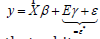
A misspecification perspective was subsequently employed for performing an eigen-decomposition uncertainty-oriented estimation analyses using the sampled, county, zip code stratified covariates. The model was built using the y = Xβ +ε * (i.e., regression equation) assuming the geosampled CRC data had autocorrelated disturbances.
Results
The county zip code geosampled CRC epidemiological data
was decomposed into a white-noise component, ε , and a set of
unspecified zip code regression models that had the structure
 in the eigen-spatial autoregressive model. We found
that white noise in a regression model was a univariate discretetime
stochastic process whose terms were independent and
independent (i.i.d.) with a zero mean. In this experiment, the
misspecification term in the county, CRC zip code prognosticative
regression model was Eγ .
in the eigen-spatial autoregressive model. We found
that white noise in a regression model was a univariate discretetime
stochastic process whose terms were independent and
independent (i.i.d.) with a zero mean. In this experiment, the
misspecification term in the county, CRC zip code prognosticative
regression model was Eγ .
The upper and lower bounds for the eigen-spatial autoregressive model matrix generated employing Moran’s I were subsequently deduced by λmax(n /1T W1 ) and λmin( n /1T W1 ) where λmax and min λ , which in this experiment were the extreme eigenvalues of Ω = HWH in the CRC stratified, epidemiological model, eigendecomposed eigen-spatial, filter, synthetic, eigen-orthogonal eigenvectors. The eigenvectors of Ω were vectors with unit norm maximizing Moran’s I. The eigenvalues of this matrix were non-asymptotically synthesizable from the semi-parameterized, diagnostic, empirical geosampled dataset, which was equal in value to the Moran’s coefficients derived from the residual eigenautocorrelation post-multiplied by a constant. Eigenvectors associated with high positive (or negative) eigenvalues have high positive (or negative) autocorrelation (Griffith 2003). The synthetic, eigen-function, eigen-decomposed, eigen-orthogonal, eigenvectors associated with extremely small hierarchical, diffusion-related, CRC, stratified, county zip code sampled estimator determinant discrete, integer values corresponded to non-zero eigen-autocorrelation (i.e., z scores >0) and were suitable for defining spatial structures corresponding to zip code aggregation / non-aggregation-oriented sites (i.e., stratified hot/cold spots of potential hyper/hypo endemic CRC patients).
The diagonalization of the geospatial uncertainty-oriented,
regression weighted matrix generated for quantitating the
autocovariance of the non-time series, dependent, potential,
spatially biased, aggregation/non-aggregation-oriented, CRC
stratified, non-zero, autocorrelated diagnostic determinants
consisted of finding the normalized vectors ui stored as columns
in the matrix U = [u1... un ], This satisfied 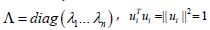 and
and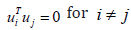 . Note that double centering of Ω implied
that the eigen-orthogonalized eigen-spatial filter eigenvectors
rendered from the eigen-decomposed, CC stratified, county, zip code
exogenous, regressors were centered, and at least one eigenvalue
was equal to zero. Introducing these eigenvectors in the original
formulation of Moran’s I in the eigen-semiparametric, eigen-spatial
autoregressive model led to:
. Note that double centering of Ω implied
that the eigen-orthogonalized eigen-spatial filter eigenvectors
rendered from the eigen-decomposed, CC stratified, county, zip code
exogenous, regressors were centered, and at least one eigenvalue
was equal to zero. Introducing these eigenvectors in the original
formulation of Moran’s I in the eigen-semiparametric, eigen-spatial
autoregressive model led to:

The autocovariance provided the covariance of the process at multiple capture points, which was closely related to the eigenautocorrelation. We centered vector z = Hx and employed the properties of idempotence of H , an equation which was then equivalent to

As the eigenvectors i u and the vector z were centered in the potential, georeferenceable, aggregation/non-aggregationoriented, hyper/hypo-endemic, county, zip code, vulnerabilityoriented, regression model, forecast equation (3.2) was rewritten:

where was the number of null eigenvalues of Ω(r ≥1) . These eigenvalues and corresponding eigenvectors were removed from Λ and U , respectively. Equation (3.3) was then strictly equivalent to:

Moreover, it was demonstrated that Moran’s I for a given
eigen-spatial filter eigenvector i u was equal to  . So, the equation was written
 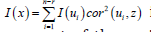 in R. The term
 represented then became part of the variance of z that
was explainable by ui in the prognosticative, CRC, regression,
epidemiological model forecasts when z = βi ui + ei . The quantity
was equal to
represented then became part of the variance of z that
was explainable by ui in the prognosticative, CRC, regression,
epidemiological model forecasts when z = βi ui + ei . The quantity
was equal to 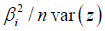 . By definition, the eigenvectors ui were
eigen-orthogonal, and therefore, regression coefficients of the linear
models z = βi ui + ei were those derivable from the prognosticative
CC regression model z=Uβ+ε=βi ui+....+βn-r un-r+ε.
. By definition, the eigenvectors ui were
eigen-orthogonal, and therefore, regression coefficients of the linear
models z = βi ui + ei were those derivable from the prognosticative
CC regression model z=Uβ+ε=βi ui+....+βn-r un-r+ε.
The maximum value of 1 was quantifiable by all the variations
of z, as parsimoniously expounded by the eigenvector u1 , which
corresponded to the highest eigenvalue λ1 in the weighted, eigenautocorrelation,
uncertainty matrix constructed from the non-time
series sampled, county, zip code estimator determinants. Here,
 and the maximum
value of I was intuitively deducible for Equation (3.4), which was
equal to
and the maximum
value of I was intuitively deducible for Equation (3.4), which was
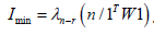
equal to 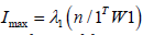 . The minimum value of I in the error
matrix was obtainable as with all the variations of z, which in this
experiment was definable by the eigenvector un-r corresponding
to the lowest eigenvalue λn-r extractable in the epidemiological
forecast model renderings. This minimum value was equal to
. The minimum value of I in the error
matrix was obtainable as with all the variations of z, which in this
experiment was definable by the eigenvector un-r corresponding
to the lowest eigenvalue λn-r extractable in the epidemiological
forecast model renderings. This minimum value was equal to
 . If the sampled, explanatory, CRC county, zip
code sampled prognosticative variable was not definable due
to the presence of heteroscedasticity, multicollinearity, or nonasymptoticalness,
the part of the variance explained by each
eigenvector was equal, on average, to
. If the sampled, explanatory, CRC county, zip
code sampled prognosticative variable was not definable due
to the presence of heteroscedasticity, multicollinearity, or nonasymptoticalness,
the part of the variance explained by each
eigenvector was equal, on average, to  . Because
the forecasted explanatory, CRC stratified diagnostic, county, zip
code, geosampled epidemiological variables in z were randomly
permuted, it was assumed that we would obtain this result Table
2-4.
. Because
the forecasted explanatory, CRC stratified diagnostic, county, zip
code, geosampled epidemiological variables in z were randomly
permuted, it was assumed that we would obtain this result Table
2-4.
Table 2: Poisson Model Summary Results.

Note: Pr(>|z|) denotes two-sided p-values from the Poisson regression. Asterisks indicate statistical significance (*p < 0.05; **p < 0.01).
Table 3: Variance Inflation Factor (VIF).

Table 4: Model Fit Parameters.


Discussion
We employed space-time model specifications, one based upon the Generalized Linear Mixed Model (GLMM), using the Moran eigenvector space-time filters to optimally quantitate violations of regression in space and geography in the multiple CRC, stratified, georeferenced racial sociodemographic and socioeconomic, geosampled, county zip code, LULC classified epidemiological observational evidential prognosticators. We identified eigenoptimization uncertainty-oriented algorithms to fit the varying stratified, forecast-oriented, county zip code stratified CRC regression model to a training dataset of non-asymptotical, multicollinear, skew heteroscedastic, zero autocorrelated estimator determinants. We were able to quantify how regression functions characterized spilled-over hierarchical diffusion of CRC in Hillsborough County at the zip code level. We were able to predictively prioritize and geospatially statistically precisely target the potential, hyper/hypo-endemic, aggregation/non-aggregationoriented, capture point, county-zip code CRC stratifiable explanatory, racial sociodemographic, and socioeconomic determinants.
The Moran spatial filtering technique employs an eigenfunction, second-order, eigen-spatial filter eigen decomposition of the REs in varying, non-temporally dependent, diagnostically stratifiable, county, zip code epidemiological sampled, racial, sociodemographic, and socioeconomic stratified estimator determinants rendered uncertainty-oriented SSREs and SURE regression components, hence denoising all the CRC stratified determinants. The Poissonian regression, spatial autocorrelation, and interpolated maps generated for Hillsborough County zip codes reveal a greater incidence of colorectal cancer in the Brandon and Riverview areas as compared to lower incidence rates in eastern Plant City, South Tampa, and northern Lutz. These localized findings are significant in comparison to previous studies that have similarly used regression modeling to assess correlations between socioeconomic status and CRC, but no study has generated zip code assessments of the incidence of CRC. Previous studies from the American Cancer Society suggest lower socioeconomic status and education levels to be statistically significant risk factors in developing CRC [21].
However, applications in Hillsborough County suggest a more complex paradigm, specifically for White Americans residing in the Brandon and Riverview area (Zip codes 33578, 33511, 33647). These findings demonstrate a higher risk for being a potential patient with CRC, as seen in Figure 3. The greater Riverview and Brandon incidence area suggests a significant need for colorectal cancer screening in this region of Hillsborough County, as compared to other regions where primary screening services may be more established. According to the National Health Resources and Services Administration, the Health Professional Shortage Area (HPSA) database is a tool used to identify primary care physician shortages across all counties within the State of Florida (HRSA, 2025) [22]. A database search on Hillsborough County HPSA designations revealed that many Federally Qualified Health Centers (FQHC), including Suncoast Community Health centers in the Brandon Riverview area, display the greatest shortages, which accounts for the red hotspot as seen in Figure 3 and greater concentration of CRC incidence in the 33511zip code (HRSA, 2025) [22].
In addition, the Tampa Family Health Centers are another widespread FQHC with this same designation, which accounts for the orange, moderate incidence of CRC as seen from Brandon to the northeast regions of Hillsborough County. With this, many white individuals in these areas had a greater, more significant risk of developing CRC as compared to other races, ethnicities, socioeconomic status, and education levels as calculated in the vulnerability index, with a value less than 0.01 indicating statistical significance. Limitations in this calculation could result from insufficient census data produced from the State of Florida, specific to Hillsborough County, but additional considerations should include access to primary care physicians at facilities with HPSA designation, nutritional accessibility, food insecurity, and previous cancer diagnosis. The middle-class white populations developing CRC at a greater rate in southeast Tampa in comparison to northern and western Hillsborough County, could be struggling with inconsistent access to HPSA primary care physicians and routine screenings.
Routine screenings beginning at age 45 - 50 are vital in the detection of early CRC developments and timely intervention, but delaying these non-invasive screenings can lead to an increased detection at advanced stages. Advanced CRC clinical presentations, such as rectal bleeding, blood in the stool, or chronic constipation, could persuade patients to visit a primary care physician if they are not already seeing their provider at least once a year, but have a great likelihood of becoming an advanced diagnosis with a greater mortality rate. This pattern of indifference in regard to primary care screenings could contribute to greater CRC incidence rates, and further stresses the need for primary care education, especially when it comes to all types of preventative cancer screenings. This data leads to the conclusion that health education, health literacy, and primary care interventions should target the Riverview and Brandon zip codes. In addition, nutritional access and food insecurity rates are critical considerations to be made in assessing CRC vulnerability.
A significant or prolonged lack of fiber in one’s diet leads to significant deficiencies and disruption of a healthy gut microbiome, which can be associated with increased risk of developing CRC. Understanding rates of food insecurity in the Riverview and Brandon areas can give greater insight into the elevated rates of CRC cancer in the region and may aid as an additional means of introducing primary interventions beyond clinical screenings. For example, local hospitals such as BayCare have implemented intake food insecurity screenings for all patients and have introduced Food Rx programs to accommodate these nutritional discrepancies (BayCare, 2025) [23]. These inventions are aimed at improving health outcomes beyond initial clinical presentation and addressing long-term health complications. Because CRC falls within long-term health outcomes, BayCare’s partnership with Feeding Tampa Bay can have a positive influence on the incidence of CRC and is a potential template for future interventions specific to the Brandon and Riverview area (BayCare, 2025) [23]. Further connections should be made in understanding the relationship between food insecurity and the greater risk and development of CRC in Hillsborough County.
Conflict of Interest
The authors declare that the study was conducted in the absence of any commercial or financial relationships that could be construed as a potential conflict of interest.
References
- Moffitt Cancer Center. (n.d.) Colon Cancer Treatment Information.
- Ahnen DJ, Wade SW, Jones WF, Sifri R, Mendoza Silveiras J, et al. (2014) The Increasing Incidence of Young-Onset Colorectal Cancer: A Call to Action. Mayo Clinic Proceedings 89(2): 216-224.
- King SC, King J, Thomas CC, Richardson LC (2025) Baseline Estimates of Colorectal Cancer Screening Among Adults Aged 45 to 75 Years, Behavioral Risk Factor Surveillance System, 2022. Preventing Chronic Disease 22: E49.
- Wang H, Roy S, Kim J, Farazi PA, Siahpush M, et al. (2019) Barriers of colorectal cancer screening in rural USA: a systematic review. Rural Remote Health 19(3): 5181.
- Rex DK, Boland CR, Dominitz JA, Giardiello FM, Johnson DA, et al. (2017) Colorectal Cancer Screening: Recommendations for Physicians and Patients from the U.S. Multi-Society Task Force on Colorectal Cancer. The American journal of gastroenterology 112(7): 1016-1030.
- Carethers JM (2014) Screening for Colorectal Cancer in African Americans: Determinants and Rationale for an Earlier Age to Commence Screening. Digestive Diseases and Sciences 60(3): 711-721.
- Pankratz VS, Kanda D, Kosich M, Edwardson N, English K, et al. (2024) Racial and Ethnic Disparities in Colorectal Cancer Incidence Trends Across Regions of the United States From 2001 to 2020 – A United States Cancer Statistics Analysis. Cancer Control.
- Florida Health Charts (n.d.). Colorectal Cancer Incidence - Florida Health CHARTS - Florida Department of Health.
- Rushton G, Peleg I, Banerjee A, Smith G, West M (2004) Analyzing Geographic Patterns of Disease Incidence: Rates of Late-Stage Colorectal Cancer in Iowa. Journal of Medical Systems 28(3): 223-236.
- National Cancer Institute. (2018) Cancer Clusters.
- He R, Zhu B, Liu J, Zhang N, Zhang WH, et al. (2021) Women’s cancers in China: a spatio-temporal epidemiology analysis. BMC Women’s Health 21(1): 116.
- Satardekar A, Liu J, McDonald H, Jacob B (2024) Employing Markov Chain Monte Carlo (MCMC) Bayesian Poissonian and a Second-Order Eigenfunction Eigen decomposition Algorithm to Geostatistically Target Landscape Covariates Associated with Leukemia in Hillsborough County, Florida. British Journal of Healthcare and Medical Research 11(4): 232-260.
- Kuo TM, Meyer AM, Baggett CD, Olshan AF (2019) Examining determinants of geographic variation in colorectal cancer mortality in North Carolina: A spatial analysis approach. Cancer Epidemiology 59: 8-14.
- Griffith D (2003) Spatial Autocorrelation and Spatial Filtering: Gaining Understanding through Theory and Scientific Visualization.
- Cressie NAC (1993) Statistics for spatial data. Revised edition. New York: John Wiley & Sons, Inc.
- Hosmer DW, Lemeshow S (2000) Applied logistic regression. 2nd edn. New York: Wiley.
- Aune D, Lau R, Chan DS, Vieira R, Greenwood DC, et al. (2011) Nonlinear reduction in risk for colorectal cancer by fruit and vegetable intake based on meta-analysis of prospective studies. Gastroenterology 141(1): 106-118.
- US Census Bureau (2020) QuickFacts Hillsborough County, Florida.
- Florida (2025) Welcome-Hillsborough.WaterAtlas.org. Usf.edu.
- com (2025) Hillsborough County Florida ZIP Codes-Map and Full List.
- Doubeni CA, Laiyemo AO, Major JM, Schootman M, Lian M, et al. (2012) Socioeconomic status and the risk of colorectal cancer: An analysis of over one-half million adults in the NIH-AARP Diet and Health Study. Cancer 118(14): 3636-3644.
- gov (2025) HPSA Find.
- org (2025) Improving Health Outcomes Year-Round: BayCare and Feeding Tampa Bay Tackle Food Insecurity and Accessibility.
-

This work is licensed under a Creative Commons Attribution-NonCommercial 4.0 International License.


