A Multilevel Hazards Model for Child Mortality in Nigeria

In this paper, we present a multilevel hazard models for factors that affects child mortality in Nigeria. These factors are in three categories; Individual level or Child level effects, Family level effects and Community level effects. Using secondary data from the National Demographic Health Survey, estimations were made employing multilevel proportional hazard model, using data that are hierarchical in nature. It is important to consider the realities of hierarchical structure of the data, especially in the Medical and Sociological studies because;

a. Focusing attention on the levels of hierarchy in the population, multilevel analysis enables researchers to understand where (in which level) and how effects are occurring.

b. It provides better estimates for answering simple questions for which single-level analysis was once used, and in addition allows for further information about the hierarchical variations to be obtained

c. Carrying out an analysis which does not recognize the existence of clustering creates serious problems. For example, clustering will generally cause standard errors of regression coefficients to be understated.

Hence, this paper investigates two parallel developments of new statistical tools for data analysis: statistical methods known as hazard models that are used for analyzing event-duration data and statistical methods for analyzing hierarchically clustered data known as multilevel models. The objective of the study is (a) To predict the death of a child at time t using Logistic regression model, (b) To compute hazard at time t of a particular child i belonging to family j in a community k from two waiting distributions (Exponential and Weibull), (c) To determine how family-level factors and communitylevel factors affects child survival, (d) To investigate child mortality at national level through the geographical zones among children in Nigeria [1].

Most of the earlier studies on Mortality have ignored the hierarchical facts. Using aggregate data often misleads the interpretation of results and therefore, we need analysis for different levels of hierarchy. However, in recent years, researchers have began to examine hierarchical effects with the help of multilevel modeling It is evident that mortality is one of the main concerns for Nigeria in which rapid population growth is taking place. According to the report of the 2011 United Nation International Children Education Fund (UNICEF 2011), the mortality rate of Nigeria is 11% of the total population [2-5]. This is a real success for a developing country (with one of the most densely populated area on earth) without significant change in economic situation.

Indicators derived from mortality rates provide a good picture of overall population health. These Indicators include infant and child mortality, adult mortality and overall life expectancy at birth. According to the World development indicators database, child mortality rate is the number of deaths of children less than 5 years old per 1000 live birth while Infant Mortality Rate is the number of deaths of children less than 1 year old per 1000 live birth. Despite its significant decline in most parts of the developed world, child mortality remains disturbingly high in most developing countries.

In Nigeria, regional disparities in mortality among children under age 5 have been reported, with higher rates observed in the Northern regions than in the Southern regions [6]. However, these were survey reports rather than empirical studies, and the role of explanatory factors was not investigated. Regional disparities in health-seeking behavior have been reported regarding child immunizations, maternal and child health care utilization, differences in the socioeconomic composition, communicable diseases, childhood nutrition, and malnutrition [7]. Other studies have reported that the Northern regions have higher proportions of home delivery and complications during childbirth, younger age of first marriage, younger age at birth of first child, and lower knowledge and use of contraception compared to the Southern regions. Regional disparities in these parameters are associated with factors at the community level that distinguish these regions from each other [8]. The reduction of these disparities is a key goal of most developing countries’ public health policies, as outlined in the Millennium Development Goals 2015.

To achieve this goal, determinants of high mortality among disadvantaged people, communities, and regions need to be identified. The physical, ecological, and political structure and impoverished socioeconomic milieu in several countries in Sub- Saharan Africa account for geographic variations in childhood mortality. One such environment is the regional environment. Poor or polluted environments tend to expose children to diseasecausing agents, predisposing them to high mortality risks. In Nigeria, marked regional disparities in mortality of children under age 5 have been reported, with higher rates observed in the Northern regions than in the Southern regions. Children in low-income countries face much higher risks of mortality compared to their counterparts in more affluent societies. While the infant mortality rate in 1992 was 79per thousand in India, it was only 26 in Thailand and 13 in South Korea. This disadvantage often arises from the lack of parental resources in societies characterized by credit market imperfections. The problem is further aggravated for larger families with more children as these families need to allocate limited available resources across more consumers. Even in the absence of any strategic behavior by family members, children compete for limited parental care and resources – a notion commonly labeled as ‘sibling rivalry’ in economics. Sibling rivalry implies that sibling composition determines child survival leading Garg and Morduch to include number of brothers and sisters or number of older brothers and sisters in a child health function. These indicators of sibling rivalry cannot however capture the intensity of competition between prior and posterior siblings. By the time a child is born, an older sibling may not require extensive care from the parents and may even help parents by looking after younger siblings or supplementing family earnings. Thus the spacing between consecutive children, i.e., the age composition of siblings could capture the intensity of competition between successive siblings better though this measure has not been adequately taken account of in the existing literature [9].

Indeed, the incorporation of community-level factors in the analysis of child mortality provides an opportunity to identify the health risks associated with particular social structures and community ecologies, which is a key policy tool for the development of public health interventions. The availability of services and social amenities in communities, or the lack thereof, may positively or negatively influence the health of the residents of communities. Some of these factors include differences in community-level development, population density, prevalence of poverty, and availability of maternal and child health care services. These are often interrelated aspects of the regional environment that are important for child health and well-being and may also be relevant in exacerbating or mitigating inequities in resources and population health outcomes across regions [10].

In recent years, all developing regions have experienced considerable improvements in child survival with Northern Africa and East Asia making the fastest progress. Despite these achievements, however, most developing countries still lag significantly behind the developed world, with an average of 66 deaths per 1,000 live births in 2009, compared to only six in developed regions and also, the annual number of children who die before they reach age five is shrinking, falling to 7.6 million global deaths in 2010 from more than 12 million in 1990 (UNICEF and the World Health Organization).

Across the world, children are at higher risk of dying if they are poor. The most impressive declines in child mortality have occurred in developed countries, and in low-mortality developing countries whose economic situation has improved. In contrast, the declines observed in countries with higher mortality have occurred at a slower rate, stagnated or even reversed [11]. Owing to the overall gains in developing regions, the mortality gap between the developing and developed world has narrowed since 1970. However, because the better-off countries in developing regions are improving at a fast rate, and many of the poorer populations are losing ground, the disparity between the different developing regions is widening.

Today nearly all child deaths occur in developing countries, almost half of them in Africa. While some African countries have made considerable strides in reducing child mortality, the majority of African children live in countries where the survival gains of the past have been wiped out, largely as a result of the HIV/AIDS epidemic [12-18]. Some developing countries still lag significantly behind the developed world, with an average of 66 deaths per 1,000 live births in 2009, compared to only six in developed regions and also, the annual number of children who die before they reach age five is shrinking, falling to 7.6 million global deaths in 2010 from more than 12 million in 1990 (UNICEF and the World Health Organization). Against this backdrop, the joint UN-World Bank report concludes that the rate of decline in child mortality remains insufficient to achieve Millennium Development Goal 4 (MDG 4)-to reduce under-five mortality rates by two thirds between 1990 and 2015.

In September 2000, the World Community adopted the Millennium Development Goals (MDGs) to re-affirm community towards a world in which sustaining development and eliminating poverty would be accorded the highest priority. All the 191 United Nations member states pledge that by the year 2015, all the MDGs consisting of a frame of 8 goals, 18 targets and 48 indicators to track progress towards the goals would be meet. The goals are quantifiable with clear cuts objectives. Goal 4 is to reduce underfive mortality rates by two thirds between 1990 and 2015. Goal 5 focuses on issues relating to maternal mortality and maternal health. Goal 6 is aimed at target in epidemiology of HIV/AIDs, Malaria and other major diseases leading to child mortality and their social consequences. It is expected that these diseases must have halted and their spread reversed by 2015 [18-23].

It is as a result of the dismal failure of meeting the public good across the developing world that the nations of the world in year 2000 met and agreed on a number of Millennium Development Goals (MDGs). Two of these goals are to reduce under-five and maternal mortality rates. But analysis of recent trends shows that Nigeria is making only marginal progress [Mid-Point Assessment Overview, MDGs Nigeria Sept 2008] in reducing these rates and attaining the MDGs even when most of the causes of these deaths are either preventable or treatable [23-26]. It is sad to note that in spite of all previous efforts, the Under 5 morbidity/mortality indices have shown only marginal reductions in the last five years, making the MDGs targets by 2015 clearly unachievable using current strategies alone.

The focus of this analysis is mortality among children in Nigeria. Since the response variable is child mortality, we utilize event history procedures to examine the effect of various factors on the risk of death of children under the age of five. A fundamental discriminating criterion between various event history models, is the distribution that the timing function is assumed to follow. In this analysis we utilize the Weibull hazard model and the Exponential hazard model.

When appropriate event-duration data are available and coupled with relevant multilevel data, survival models provide the best strategy for analyzing processes of qualitative changes in states (transitions) and their multilevel determinants in terms of fixed and random parameter variations across individuals and groups. A weakness of this approach is that time is used as another explanatory variable without its recognition as the domain in which qualitative changes in states takes place in a dynamic way within specific contexts.

Let there be N state an individual can occupy at any moment of time in a given context. Suppose that there are three levels (i, j and k) of hierarchically-clustered data for a sample of individuals (e.g. a sample of children nested within families and families nested within area of residence or communities). Let be the survival time that elapses before the i-th child (level 1) belonging to the j-th family (level 2) in the k-th area of residence or community (level 3) makes a transition from state l to state m. In a single-level analysis, if individuals initiate the failure time process in a state l, there are N-1 latent time with densities

Where f ^lm (.) is the density function of times to transition from state l to state m, h^lm (.) and is the associated hazard function.

The joint density function of the (N-1) latent transition times is given by

In a three-level frame work considered above, let ε_ijk, ϑ_jk and θ_k be the random coefficients at the child level, the family level and the community level respectively. Ignoring the multi-state situation, if the random effects are assumed to operate multiplicatively on the baseline hazard, they are interpreted as relative risks and the general multi-level hazard model can be written as follows:

Where

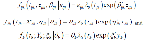
Where Z_ijk is a 1 x K vector of level-1 exogenous (time-invariant or time varying) variables associated with survival time t_ijk for the i-th child belonging to the j-th family living in the k-th area of residence or community. β_ijk is a K x 1 vector coefficient that may represent both fixed effect and random effect of explanatory variables.X_jk is a 1 x L vector of level-2 exogenous (time-invariant or potentially time-varying) variables associated with survival time t_jk for the j-th family living in the k-th community. η_jk is a L x 1 vector of associated coefficient that may represent both fixed effect and random effect of explanatory variables. Y_k is a 1 x M vector of level-3 exogenous (time-invariant as well as potentially timedependent) covariates.ξ_k is a M x 1 vector of associated coefficients.

Following the multilevel hazard model can be parameterized in a general way (without level-specific or cross-level interactions) and written as;

Where is the unknown duration dependence?

This general formulation allows ε_ijk, ϑ_jk and θ_k to be function of time. By exponentiating the term in brackets, equation (4) ensures that the hazard function is positive as required since it is a conditional density function. From the multilevel survival formulation in (4), the survivor function at time t is;

and the likelihood is more generally:

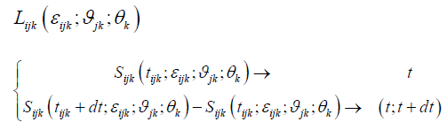
Where t= if the spell censored at time t

(t; t+dt) =if the event occurred at time t

We consider a three-state process of infant and child mortality, a non-repeatable event. The two states that a child can occupy during the time of interview are ‘alive’ and ‘dead’. Note that a child can exit the alive state only once after a given length of exposure to the risk of death. There are thirteen factors to measure the survival status of a child from birth to age five. My focus is on hazard process in which one or more covariates change values between intervals but are constant within an interval (i.e one or more covariates are time-varying).

Here we look at a situation where there are several children per family. In practical terms, at each month of exposure t, we can define a response variable for each child i belonging to family j in a k community,

Where 1=if child i dies before month t

0=if child i survive beyond month t

Where is 5 years.

let P_ijk denotes the response probability of the i^th chaild of the j^th family in the k^th community that survive up to age 5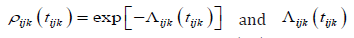

Table 1: Data Organization for Hierarchically Clustered /Multilevel Data.

For a simple illustration, suppose we have four families (mothers) in four different communities, the first mother from the first community has two children, with the first child dying at 5th month, and the second censored at 2 months. The second mother from the second community has one child censored at 2 months, the third mother from the third community has one child censored at 4 months and the fourth mother from the fourth community has one child dying at 4 months (Table 1).

The survival times for a hierarchically clustered sample of individuals are assumed to be conditional on two independent cluster-specific random effect, θ_k and ϑ_jk . We assign one θ_k random effect to each of the k=1…K clusters, ϑ_jk one random effect to each of the j=1…J, sub-clusters of cluster θ_k . Since the data are hierarchically clustered, all individuals in the j-kth sub-cluster are member of one and only one type-k cluster. Let t_ijk represent the survival times that elapses before the i-th child (level 1) belonging to the j-th family (level 2) in the k-th community (level 3) and let x_ijk represents a vector of covariates for the ith member of this cluster. If the random effects are assumed to operate multiplicatively on the baseline hazard, they are interpreted as relative risks and the model is written as

Where λ₀ t(_ijk) represents the baseline hazard, which we assume to be piecewise constant, and exp( ) (α ′x_ijk) is the risk associated with covariates x_ijk .

Individuals who have died (Y_ijk =1) contribute to the conditional likelihood function, the product of the conditional hazard and the conditional survival functions, while individuals whose survival times are censored (Y_ijk =0) contribute to the conditional survival function:

Here, integrated hazard corresponding to We will omit the arguments when referring to the hazard and the integrated hazard and denote these quantities simply as We can write the ith cluster’s contribution to the conditional likelihood function as,

Note that once we condition on the unobserved random-effects, the individual observations in the sample are independent.

If the frailty effects θ_k and ϑ_jk were observed, and their distributions were known, one could estimates the parameters of these models by miximising eqn (6) with respect to , ξ_k, η_jk and β_ijk here are the parameters of the two mixing distribution and ijk β is a vector consisting of the covariate effects, α_ijk , and parameters that specify the baseline hazard. Since these quantities are not observed, we must either integrate them out of the likelihood function or use the Expectation-Miximization (EM) algorithm and we must make assumptions about the probability distributions of the two random-effects

We assume that the random effects are independent and are Exponentially distributed with density functions,

The variances for the above distribution are ξ⁻² and η⁻² respectively and their covariances will be estimated. The assumption of the random effects being exponential and weibull follows a previous reserch. The estimated parameters describing the shape of the weibull-distributed random-effects can be interpreted in several different ways. The most direct interpretation is simply as the variance of the frailty distribution, if the variance is zero, then observations from the same group are independent. A larger variance implies greater heterogeneity in frilty across and greater correlation among individuals belonging to the same group. The second way to describe the results is to construct a risk ratio that compares the conditional expectation of the frailty-effect for a high-risk group and a low-risk group, where for instance, high-risk may refer to a cluster at the 90th percentile and low-risk a cluster at the 10th percentile of the frailty distribution.

As the variance of the random effects tend to zero, the observations in each cluster becomes progressively less correlated. Full independence among all observations in the sample is obtained in the limiting case. Under full dependence, the multilevel hazard model simplifies to Guo and Rodriguez’s (1992) multivariate hazard model with a single random-effect. If the variance of one of the two random-effects is sufficiently small, the parameter estimates and standard errors in the multilevel model differs little from those estimated using a standard hazard model. Estimating a simpler model is desirable because of the time and computational effort required to estimate the random-effects models, particularly the multilevel model. In addition, as the variance of the random effects becomes difficult-and eventually impossible-to evaluate the numerical integration procedure and certain functions that are part of the estimation procedure.

The values for θ_k and ϑ_jk that appear in the likelihood function are unobserved. One method for obtaining maximum likelihood estimates of ξ_k, η_jk and β_ijk under these circumstances is to apply the Expectation Maximization (EM) Algorithm (Dempster, Laird and Rubin, 1977). One can also obtain direct maximization using the Newton-Raphson method which requires the first and second derivatives of the incomplete data log-likelihood function to be evaluated at each iteration using numerical integration techniques. An iteration using the Newton-Raphson method is given by,

Where ϕ_n represents the parameters of the model at the nth iteration; F_n is a vector of first derivatives and H_n is a matrix of second derivatives, both evaluated at ϕ_n . Under the Newton- Raphson method, there is need for a second derivative of the incomplete data log-likelihood. However, the matrix of second derivatives that are calculated as part of the Newton- Raphson procedure provides estimates of asymptotic variance. Finally, the Newton-Raphson method generally enjoys rapid convergence.

Finally, the calculation of the first derivative of the incomplete data log-likelihood function at each iteration is more computationally intensive.

In this section, the proposed methodology to data collected from three hierarchical levels in child mortality is applied. The performance of alternative methods to estimating parameters of models with data on child mortality that are clustered was also used. This study was designed to determine those factors that affect the survival of children in Nigeria and to also examine the cluster that is being affected. Most commonly, clustering occurs as a result of sample design that focuses on community or village, mothers or households, and on all the children associated with them so as to measure the extent to which risk of death of children belonging to the same household and community are correlated.

From fig 1 below, we can see that there are more deaths in the rural area than in the urban area. The reason for this increase is the fact that children suffer from social infrastructure and services like (schools, roads, electricity, and health services). Some other identifiable cause of child mortality can also occur from parent unemployment, social deprivation, and endemic conflict, in the rural area than in the urban area (Figure 1).

On geo-political zones basis (Figure 2), the North West has the highest mortality rate, followed by the North East, North Central, South South, South West and with South East carrying the least. The reason for these differences is that we have higher proportion of children in the Northern zones who have never received vitamin A supplements and immunization. Also breastfeeding rate in these zones is lower than in the Southern zones, as is the proportion of children who received complementary feeding. Use of uniodized salt is also more common in the Northern part of Nigeria. Identifiable causes of death in these area are diseases like Malaria, Vaccine preventable diseases particularly measles, pneumonia, diarrhea, and Neonatal Jaundice. Increased in prices of food and poor households became more and more food insecure. The most food insecure households were located in the Northern region where the childhood mortality indices were also high. Children in poor Nigerian households are chronically undernourished, suffering a recurrent lack of access to food of sufficient quality and quantity, good healthcare, and necessary caring practices(Figure 2).

From the survival graph below (Figure 3), we can see that the hazard rate for Exponential distribution is constant over time. This means that on average 0.5 events will occur per individual at risk per month (during a period in which the hazard remains constant at this value). The survival rate for exponential declines monotonically with time (i.e the risk of a child dying decreases with time). We can infer that the risk of death occurring among Underfive children decreases with time. This situation is referred to as Negative Duration Dependence(Figure 3).

For the Weibull distribution in Figure 4, both the hazard rate and the survival rate declines monotonically with time. We can also infer that the risk of under-five mortality decreases as time increases. This will make the United Nations MDGs: to reduce under-five mortality to 2/3 by 2015 achievable(Figure 4).

Table 2: Hazard model results for exogenous demographic and house hold socio-economic covariates in Nigeria (with P-values in parentheses).

In Table 2 below, we estimated four different models specifications using the Weibull distribution only. Model 1 is a standard hazard model with no correction for clustering. Model II is hazard model with clustering at child level, Model III is hazard model with clustering at Family level, and Model IV is a hazard model with clustering at the community level. The results indicate that there is standard relationship between child mortality risk and the covariates itemized in this sample. From the result obtained, we discovered that nearly all covariates are statistically significant and the estimated effect for the proximate determinant are in close agreement with what we have in open literature and other research studies. Based on the multilevel results, we discovered that mortality variables at the family and community levels are more statistically significant with their p- values less than 0.5, which implies that child survival is most controlled or determined by Family and Community levels and that variables at the Child level is not weighty (Table 2&3).

Table 3: Two-Level Two-State Parametric Hazard Models of Determinants of Infant and Early Childhood Mortality in Nigeria.

Table 3 shows the result of the conventional parametric hazards model (without random effects) as well as those of twolevel parametric hazards model (with random effects). These two levels hazard models contain both fixed and random effects. The fixed effects are in the first part of the table and the random effect in the second part. The fixed effect represents the population mean influences on infant and early child mortality specific to the measured covariates. The child specific random effect captured by the unobserved heterogeneity consists of two components, a measurement error plus the actual variability (heterogeneity) in child specific capacity to survive during the for the five years interval. Some of this variability may be genetic unobserved or unmeasured by the survey. Note that the frailty effects are significantly different from zero. In other words, there are unmeasured child-specific randomly varying risks that affect child survival independently of measured risk factors. Failure to account for such childspecific unmeasured characteristics has several consequences. First, ignoring individual frailty leads to underestimating the standard errors of parameter estimates, creating false impression of precision. An examination of each of the parametric models (exponential, Weibull) under single-level and two-level specifications consistently substantiates the underestimation of all standard errors under the single-level modeling scheme, and confirms the consequences of ignoring random effects in modeling Multilevel Hazard model for Hierarchically clustered data. Second, estimates of the baseline hazard duration pattern might be biased in downward direction (the best way of understanding this is by imagining a process of constant hazard). Third, estimates of covariates may be biased. The comparative results show that while the sign of most parameters are unaffected by randomly varying risk of mortality, their magnitude and level of significance are quite affected when frailty is explicitly modeled (Table 3).

The result in Table 3 below shows the conventional parametric hazards model (without random effects) as well as those of twolevel parametric hazards model (with random effects). These twolevel hazard models contain both fixed and random effects. The fixed effects are in the first part of the table and the random effects in the second part. The fixed effects represent the population mean influences on infant and early child mortality specific to the measured covariates. The child-specific (or within child) random effect captured by the unobserved heterogeneity consists of two components, a measurement error plus the actual variability (heterogeneity) in the child’s capacity to survive during the month of survival. Some of this variability may be genetic, unobservable or unmeasured by the survey. As seen in Table 2, the general findings are consistent with evidence generated elsewhere: the protective effects of full immunization status, breastfeeding (especially full breastfeeding), possession of modern amenities and increased household income, and the deleterious effects of overcrowding, closely spaced births and low birth weight. Note that the frailty effects are significantly different from zero. In other words, there are unmeasured child-specific randomly varying risks that affect child survival independently of measured risk factors. Failure to account for such child-specific unmeasured characteristics has several consequences. First, ignoring individual frailty leads to underestimating the standard errors of parameter estimates, creating false impression of precision. An examination of each of the parametric models (exponential, Weibull) under single level and two-level specifications consistently substantiates the underestimation of all standard errors under the single-level modeling scheme. Second, estimates of the baseline hazard duration pattern are biased in downward direction (the best way of understanding this is by imagining a process of constant hazard). Third, estimates of covariates may be biased. The comparative results show that while the sign of most parameters is unaffected by randomly varying risk of mortality, their magnitude and level of significance are quite affected when frailty is explicitly modeled.

Many researchers have devoted considerable attention to the impact of individual-level factors on child mortality, but little is known about how family and community characteristics affect health of children. Trend in child mortality as well as its determinants, has long been the subject of academic and policy debates. In spite of this, the problem of child mortality remains as daunting as ever. In fact, advancement in medical sciences and the upsurge in information and telecommunication technology equipment have not significantly reduced child mortality in the country, unlike in the West.

None

No conflict of interest.

1. Kalbfleish JD, Prentice RL (1980) The Statistical Analysis of Failure Time Data. New York: John Wiley, USA.
2. Cox DR, Oakes D (1984) Analysis of Survival Data, New York: Chapman and Hall, USA.
3. Guo G, Rodriguez G (1992) Estimating a multivariate proportional hazards model for clustered data using the EM algorithm, with an application to child survival in Guatemala. Journal of the American Statistical Association 87(42): 969-976.
4. Curtis SL, Diamond, McDonald JW (1993) Birth interval and family effects on post neonatal mortality in Brazil. Demography 30(1): 33-34.
5. Santa Monica (1995) A multilevel hazards model for hierarchically clustered data: Model estimation and an application to the study of child survival in Northeast Brazil.
6. Yang M, Goldstein H (1996) Multilevel models for longitudinal data.
7. Kuate Defo B (2001) Modeling Hierarchically Clustered Longitudinal Survival Processes with application to Childhood Mortality and Maternal Health 28(2): 535-561.
8. Cesar CC, Palloni A (2004) Analysis of Child Mortality with Clustered Data: A Review of Alternative Models and Procedures. Center for Demography and Ecology, University of Wisconsin-Madison, 97-04.
9. John Fox (2006) Introduction to Survival Analysis Harttgen, Kenneth: Misselhorn, and Mark: A multilevel approach to explain child mortality and under-nutrition in South Asia and Sub-Saharan Africa, 152.
10. Omariba DWR (2004) Family Level Clustering of Childhood Mortality in Kenya. 04-09.
11. Kirosa GE, Whiteb MJ (2004) Migration, community context, and child immunization in Ethiopia, 2603-2616.
12. Boco AG (2010) Individual and Community Level Effects on Child Mortality: An Analysis of 28 Demographic and Health Surveys in Sub- Saharan Africa, 72.
13. Chung MK, Shu-Chen HW, Herrin GD (1986) The use of a mixed Weibull Model in occupational injury analysis. Elsevier Science Publishers B.V., Amsterdam - Printed in The Netherlands. Journal of Occupational Accidents 7 (1986): 239-250.
14. Gardiner JC (2010) Survival Analysis: Overview of Parametric, Nonparametric and Semi-parametric approaches and New Developments Division of Biostatistics, Department of Epidemiology, Michigan State University, East Lansing, MI 48824: 252-2010.
15. Reto Schumacher (2011) Infant and early childhood mortality in a context of transitional fertility. Geneva 1800-1900: 15-16
16. Beale EML (1977) Discussion of Maximum like hood estimation from incomplete data via the EM algorithm. Journal of the Royal Statistical Society, Series B, 39: 22-23.
17. Berndt EB, Hall HR, Hauseman J (1974) Estimation and inference in nonlinear models. Annals of Economic and Social Measurement 3: 653-665
18. Clayton DG (1978) A model for association in bivariate life tables and its application in epidemiological studies of familial tendency in chronic disease incidence. Biometrika 65(1): 141-151.
19. Clayton DG, Cuzick J (1985) Multivariate generalizations of the proportional hazards model (with discussion). Journal of the Royal Statistical Society Series A 148: 82-117.
20. Kalbfleisch DJ, Prentice RL (1980) The Statistical Analysis of Failure Time Data. New York: Wiley.
21. Goldstein H (1999) Multilevel Statistical Models, Internet Edition. London: Arnold.
22. Sastry N (1997) A nested frailty model for survival data, with an application to the study of child survival in Northeast Brazil. Journal of the American Statistical Association 92(43): 426-435.
23. Snijders T, Bosker R (1999) Multilevel Analysis: An Introduction to Basic and Advanced Multilevel Modeling. Thousand Oaks: SAGE Publications.
24. Mesike, C Godson (2012) Environmental Determinants of Child Mortality in Nigeria, 5(1).
25. Guo SW, Lin Y (1994) Regression Analysis of Multivariate Grouped Survival Data. Biometrics 50(3): 632-639.
26. Kwok OM, Underhill AT, Luo W, Yoon M (2009) Analyzing Longitudinal Data with Multilevel Models: An example with Individuals Living with Lower Extremity Intra-Articular Fractures. Rehabil Psychol 53(3): 370- 386.