A Nonparametric Random-Effects Meta-Analysis Model for Diagnostic Accuracy Studies with Multiple Thresholds of Quantitative Biomarkers

Introduction

Steinhauser et al [1] developed a method for the meta-analysis of multiple diagnostic test accuracy studies of a quantitative biomarker that reported sensitivity- and specificity-values at multiple thresholds of the biomarker. Their method is implemented in a user-friendly and free [2] and is very quick, depending a little bit on choice of the specific model and size of the data. Steinhauser et al made specific choices for the analysis model which validity may be questioned for some biomarkers. Their first choice concerned the distributions of the biomarker, which was assumed to be either normal or logistic. Obviously, this assumption may not be valid in particular cases. Second choice concerned the application of standard linear mixedeffects regression models of transformed sensitivity- and specificity- values on the biomarker-thresholds. The assumption about the linear relationship between transformed sensitivity and specificity and thresholds need not be correct. Lastly, the residuals of the models for transformed sensitivities/specificities associated with different thresholds in the same study (i.e., e_si and f_si in the Steinhauser paper) were assumed to be independent. This assumption is peculiar because different realisations of the sensitivities/specificities in the same study are almost certainly correlated (with increasing threshold, sensitivity will -necessarily- decrease and specificity will similarly increase). A final concern is that the method is based on the normal distribution approximation of the binomial distribution of the numbers of true positives and true negatives (with the usual 0.5-trick when sensitivity or specificity is zero or 1). Steinhauser et al did point to this concern but did not as yet implement the binomial distribution of sensitivity/specificity in their R-package.

To address these issues we extended the work of Steinhauser et al for data of the type that was considered by Steinhauser et al. We suggest to use a nonparametric method based on the multinomial distribution. In the next sections we elaborate the type of (meta-) data we aim to analyse, we specify our statistical model and estimation method. To illustrate we show results of two data sets; a new set concerning results on the enhanced liver fibrosis (ELF) biomarker that might be useful to diagnose advanced liver fibrosis and a set that was published by [4] on diagnostic accuracy of fractional exhaled nitric oxide for the diagnosis of asthma. We finish with a discussion section.

Materials and Methods

Type of data

We consider a series of N diagnostic studies of a quantitative biomarker Y. In study i there were included n_i1 ‘cases’ and n_i0 ‘controls’. In the report of study i the sensitivities and specificities to distinguish cases and controls were reported for k_i different cutoff-values (ki≥1):ξ_i1,ξ_i2,....,ξ_iki Hence, for cutoff-value ξ_ij the observed sensitivity- and specificity-values were se_ij and sp_ij (see Table 1 with example data). From these reported results we calculated in every study the observed numbers of cases and controls with biomarker-values in between cutoff-values: y_i1j=n_i1(se-1-se_ij) is the number of cases with ξ_ij-1< Y ≤ ξ_ij and y_i0j=n_i0(sp_i,j+1-sp_ij)is the number of controls with ,ξ_i,j-1< Y≤ ξ_ij. Sensitivity se_i0 and specificity sp_i,ki+1 were defined as zero and could therefore be considered to be associated with cutoff-values ξ_i0=-∞ and ξ_i,ki+1 = ∞ , or any biological or theoretical lower- and upperbound of Y .

So, for study i we translated published results into a vector of observed numbers of cases in the k_i+1 categories of Y in study i , denoted as y_i1=(y_i10,...,y_i1ki) and a vector of observed numbers of controls in the same k_i + 1 categories of Y , denoted as y_i0=(y_i00,...,y_i0ki). It is important to stress that in general the number of cutoff-values,k_i , (likely) varies between studies and also that the specific cutoff-values themselves, ξ_i1,....,ξ_i,ki , vary between studies. It is also important to stress that the biomarker Y is represented in this way as a categorical variable through the cutoff-values, and that the k_i+1 categories can be considered as ordered

Statistical models

We considered the distributions of the vectors y_i1 and y_i0 to be multinomials given the numbers of cases and controls:

are vectors of length k_i+1 of probabilities:  π_i1j and  π_i0j are the probabilities that a random case or control in study i had biomarker value ξ_ij-1< Y ≤ ξ_ij Notice that in this model the covariance between two realisations y_{i1 j} and y_iil in the group of cases in study i equals −π_i1j π_i1l/n_i1 (and similarly in the group of controls), and therefore the asymptotic covariance between for instance se_i1 =π_i1 and se_i2 =π_i1+π_i2 is equal to se_i1(1-se_i2)/n_i1 − se n , which is not necessarily zero (as is assumed in the diagmeta-package by Steinhauser et al).

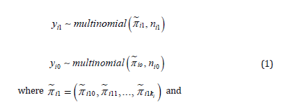
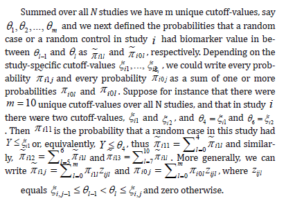
There are several options to further model π_i10,π_i11,...,π_i1m and π_i00,π_i00,...,π_i0m and we explored two ways, namely by mixing the multinomial distributions with a multivariate normal or with the Dirichlet distribution. For the multinomial-normal mixture we first transformed πi10,πi11,...,πi1m and π_i00,π_i00,...,π_i0m using the soft-max transformation as:

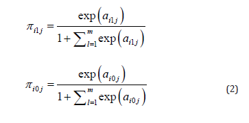
(and a_i10 = a_i00 = 0 ), and then we assumed that the vector of parameters of study ωi=(a_i11,....,a_i1m,a_i01,...,a_i0m), was a random draw from the multivariate normal distribution with mean μ (of length 2m) and covariance matrix Σ (of dimensions 2m). With this assumption our model is a random-effects meta- analysis model. A fixed-effects model is obtained by assuming Σ = 0 , or actually by constraining a_i1j =a_1j and a_ioj=a_oj for all i .

This model is an extension of the bivariate meta-analysis model. If there is only one cutoff-value (θ ) , then π_i10,π_i00,π_i11 are the probabilities of false negative, true negative, true positive and false positive outcomes in study i , respectively, and i11 a and i01 a are the logit-transformed sensitivity and 1-specificity of study i . In such case the parameter μ represents the average logit-transformed sensitivity and 1-specificity in the population of diagnostic accuracy studies of this biomarker [3].

Like the bivariate model, our extended model can be generalized with (study-specific) covariates, and given the ordinal character of the biomarker categories it seems sensible to use a ordinal logistic model, such as for instance a proportional odds model:

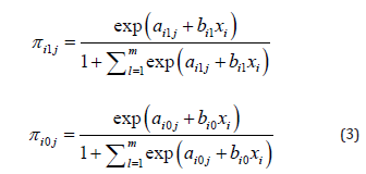
where xi is the observed value of a vector of covariates of study i . The vector of covariates may be different for cases and controls and the values of the covariates may even differ between biomarker- categories. The regression coefficients β_1i and β_0i may also vary over categories of the biomarker, but then the ordinal character of the biomarker-categories is not used in the statistical modeling. It may be useful too to assume that these regression coefficients are fixed parameters and not vary over studies (i.e.β_i1 = β₁ and β_i0 = β₀ for all studies). For now we will consider the situation without covariates.

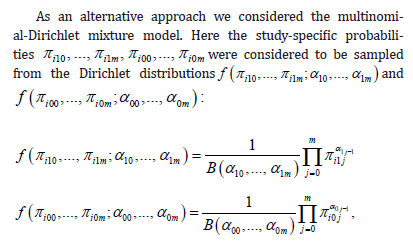
where B(…) are beta-functions. This mixture model is also a random-effects meta-analysis model. Notice that the study-specific probabilities of cases (π_i1j) and of controls (π_i0j) were supposed to be drawn from different Dirichlet distributions. This was chosen because of ease of computations, but is not absolutely necessary. It is different from the multinomial-normal mixture that is specified above, where a_i0j and a_i0j were sampled from a single multivariate normal distribution, but that choice can be amended too by drawing a_i1j and a_i0j from different normal distributions. The multinomial- Dirichlet mixture model can also be generalized to include covariates (by modeling α_1j and α_oj as functions of covariates x ), but here we only considered the model without covariates.

Estimation

We first considered the multinomial-normal mixture model. Given ω_i=(a_i1,a_i0) the conditional log likelihood of (y_i1,y_i0) equals

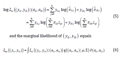
where

is the multivariate normal distribution function with mean and covariance matrix Σ . Summing contributions over all N studies gives the total marginal log-likelihood.

The integral in the marginal likelihood is multidimensional of dimension 2m and has no analytical solution. Optimizing the total log marginal likelihood is difficult if m is large, therefore based solely on convenience-arguments we decided to use MCMC-methods in a Bayesian framework to estimate the parameters of interest, i.e., ( ) 0 1 μ = π ,π andΣ (where 0 π and 1 πare the vectors of category- probabilities averaged over studies for controls and cases, respectively). In this framework we used as hyperprior distributions

where S was a diagonal symmetric matrix with entries ”0.001”, and R was a diagonal symmetric matrix with entries ”1”. These hyperprior distributions were considered to be (almost) uninformative.

The model was implemented in JAGS [7] and was run through the R-interface of JAGS. Below is the JAGS-syntax in the Additional Material-section. We chose to apply 50.000 burn-in iterations and then checked convergence. When converged we drew 50.000 val ues from the posterior distributions with a thinning parameter of 10 to reduce autocorrelation between sampled values. Afterwards the posterior distributions were graphically illustrated and summarised with the mean, median and 2.5^th and 97.5^th percentiles. We also derived posterior distributions of transformations of (π 0 ,π1 ) , such as sensitivities, specificities and Youden index values.

Estimation of the multinomial-Dirichlet mixture was slightly easier because integrals involved in the likelihood can be solved analytically. Given ( 10 ,...,  1 ) π i π i ki the conditional likelihood of ( ) 10 1 ,..., i i ki y y equals

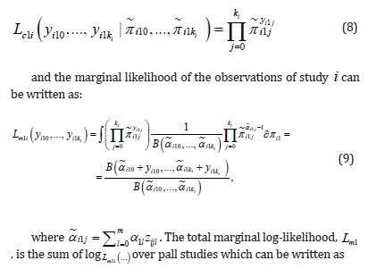
A similar total marginal log-likelihood was obtained for the data of the control-subjects in the N studies. These two likelihoods were independent, hence the decision to use two Dirichlet distributions led to separate analyses for the case- and control-data.

Like with the multinomial-normal mixture we used MCMC- methods in a Bayesian frame-work to estimate the parameters of interest in this approach too, i.e.,α₀₀,....,α_0m and α₁₀,...,α_1m . Convenient is the possibility to obtain posterior distributions of any function of α₁₀,...,α_1m and α₀₀,....,α_0m, such as averaged category-probabilities for cases and controls, sensitivities, specificities and Youden-index values. In this frame-work we used as hyperprior distributions independent gamma distributions: α_1j gamma , and α_0j  gamma for all j = 0,..., m).

Results

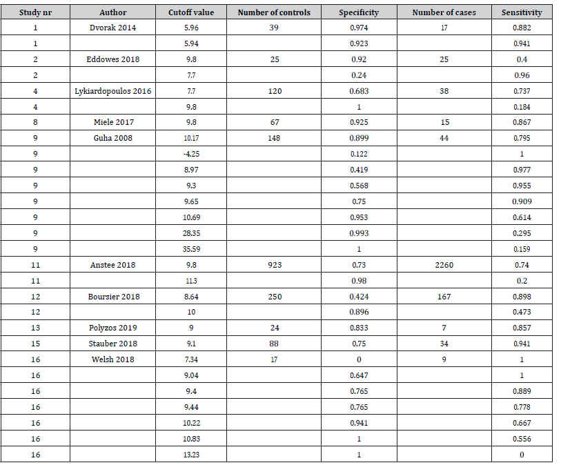
We analyzed data coming from N = 10 studies on the diagnostic value of the enhanced liver fibrosis (ELF) biomarker for diagnosis of advanced liver fibrosis. ELF is a weighted combination of type III procollagen peptide (PIIINP), hyaluronic acid (HA), and tissue inhibitor of metalloproteinase-1 (TIMP1) measured in blood. The data retrieved from the 10 published papers is summarised in Table 1. Results are available of 28 study-specific cutoffs and m = 24 unique thresholds of the ELF biomarker.

Table 1:Study cutoff values, and observed sensitivities and specificities in the various studies on the diagnostic value of the enhanced live fibrosis (ELF) biomarker.

Using the multinomial-normal mixture approach, estimated averaged category-probabilities (i.e., 1 for cases and 0 for controls) were calculated and those are reported in the top panel of Figure 1: on visual inspection the biomarker did not seem to be normally distributed, especially not in the controls. The empirical cumulative distribution functions are illustrated in the lower panel of Figure 1, separately for the cases and the controls. In these figures every study is represented by colored thin lines, and the averaged cumulative distribution functions are represented by thick black lines.

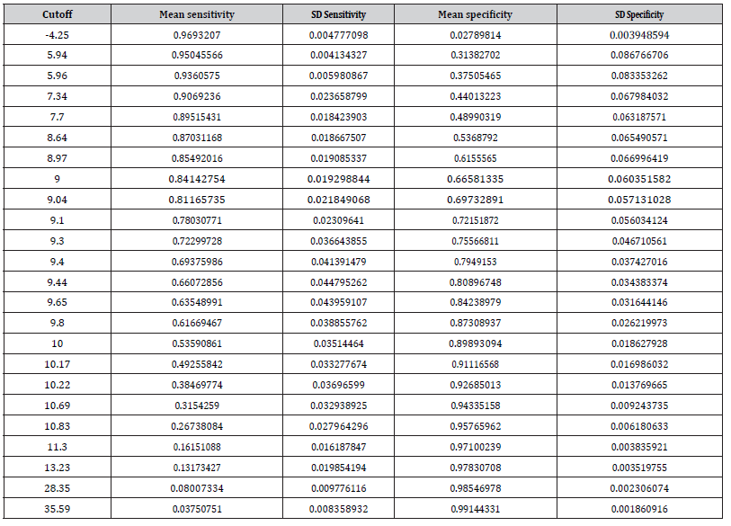
From the estimated average distribution functions we calculated the average ROC curve and the average Youden index-values for all thresholds. Both are given in Figure 2. Youden index was highest for the cutoff-value Y=9.8 (Youden index=0.49, 95 % CI: 0.437-0.541), but a similar value was found for Y=9.0 (Youden index= 0.488, 95% CI: 0.383-0.606). Estimated averaged sensitivities and specificities for all unique thresh-olds are reported in Table 2.

Table 2:Cutoff values and estimated averaged sensitivities and specificities.

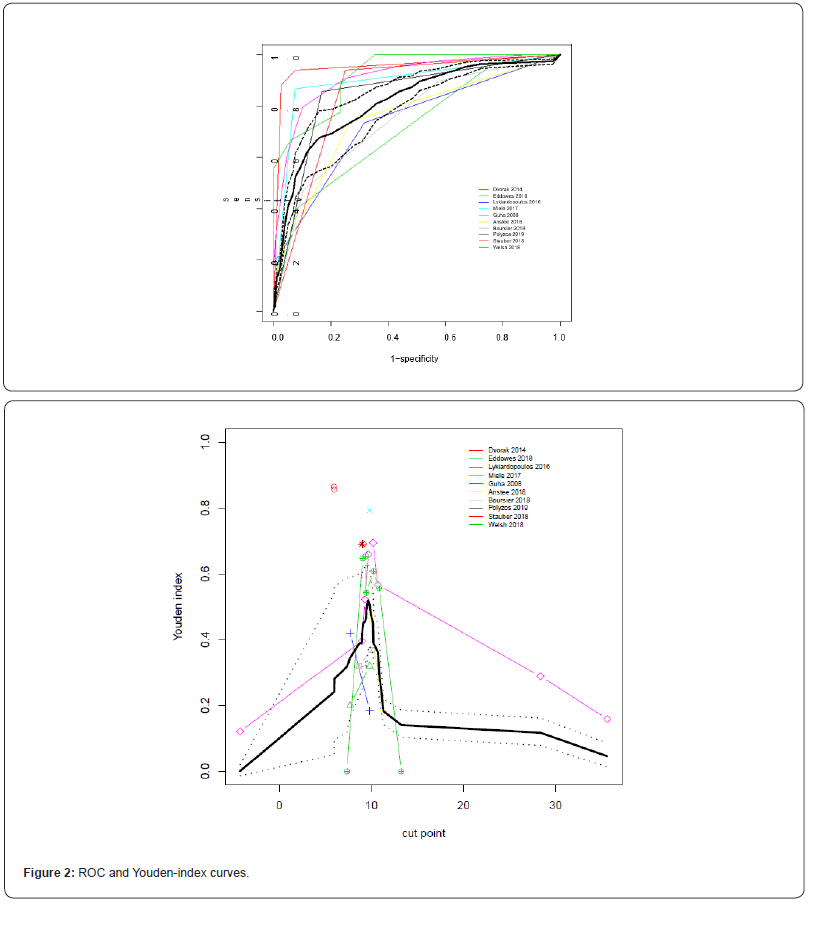
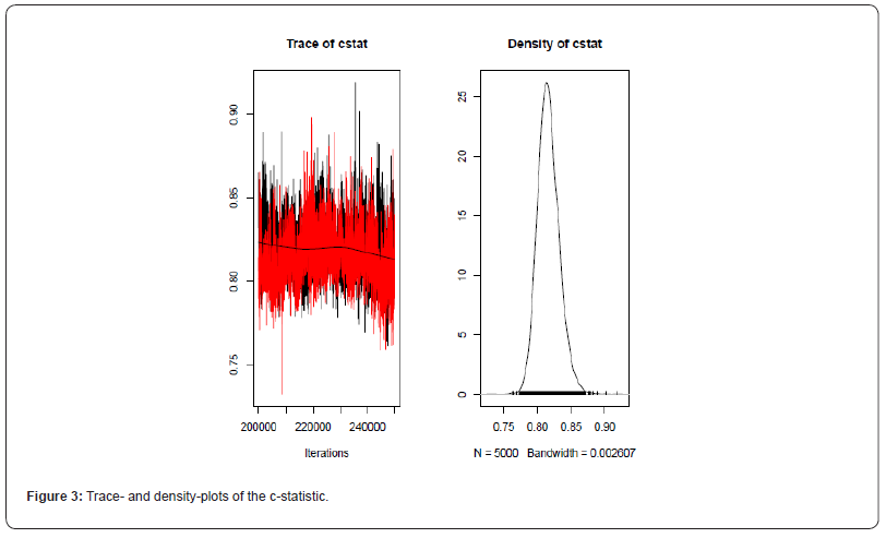
The area under the ROC (AUC) was estimated as 0:816 with 95% credibility inter-val 0:788 0:851. Convergence of the model seemed to be sufficient; as an exam-ple the trace- and density-plots of the AUC-statistic are given in Figure 3. Using the multinomial- Dirichlet mixture we found similar results, although in general with wider credibility intervals; estimated area under the ROC was 0:792 with 95% credibility in-terval 0:700 0:866. Estimated area under the ROC was 0.796 (95% ci: 0.68-0.88) according to the least constrained DIDS model of Steinhauser et al, but the DIDS algorithm did not converge. Only with the simpler CS- and CI-models did their algorithm converge but then the AUC estimates were 0.747 and 0.696, respectively.

As a second example we re-analyzed the data of [4] on the diagnostic accuracy of fractional exhaled nitric oxide (FENO) for the diagnosis of asthma. The data were from 29 studies reporting sensitivity and specificity results of 150 cut-offs, of which 53 thresholds were unique. The data is available on: https://data.mendeley. com/datasets/fndpn5bnps/1.

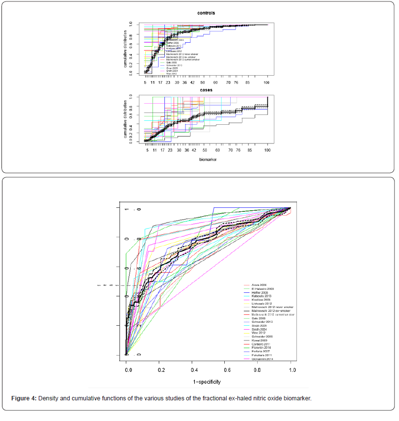
The random-effects model did not converge within a reasonable time-frame, and therefore we performed a fixed-effects analysis. The results of the multinomial-normal and of the multinomial- Dirichlet mixture models were again very comparable; we report therefore only the results of the multinomial-normal mixture model. Observed and estimated average cumulative distributions of FENO in controls and cases per study are reported in Figure 4 (top panel) and the associated ROC curves are reported in the lower panel. The thin coloured lines are associated with the individual studies, the thick black lines represent averages (together with 95% credibility intervals). Area-under-the-averaged-ROC-curve (AUC) was estimated as 0.750 (95% CI: 0.732-0.767). AUC was estimated as 0.778 (95% ci: 0.710-0.834) according to the DIDS-model of Steinhauser et al [5].

Discussion

We extended the work of Steinhauser et al for the meta-analysis of the results of a series of diagnostic studies of a quantitative biomarker Y where results were reported with sensitivity and specificity values at multiple and varying cutoff-values across the studies. Our model is based on the observed numbers of cases and controls in the various categories of the biomarker Y defined by the cutoff-values used by the different studies and we specified a random- effects, meta-analytic, structure. Our approach gave similar results as Steinhauser et al’s method for the two example datasets that we considered, but that may not be the case in general. Our model requires less assumptions and therefore is likely more robust.

Both our and Steinhauser et al’s method ignore the reasons why the specific cutoff-values were chosen in the studies, so, basically, the cutoff-values were considered to be ‘fixed’. In practice cutoff- values are probably highly coincidental and the sampling-variation underlying these choices is ignored, which likely leads to too small credibility or confidence intervals.

That our approach does not require any distributional assumption for the biomarker is a nice feature, but it has as a downside that statistics (like Youden, sensitivity, specificity) can only be calculated for cutoff-values that have been used in at least one study. This is unlike Steinhauser et al’s method where the underlying parametric model also allows estimation of performance statistics at thresholds that not have been used by any of the included studies. Our model can perhaps be smoothed in order to facilitate interpolation, for instance by penalizing squared differences between adjacent categories (i.e.,π_i1j−π_i1,j-1)² − ), but that is outside the scope of the present paper.

Our approach is implemented in the standalone computerprogram JAGS and runs through the rjags-library in R. It is much less fast than the approach of Steinhauser et al, needing hours of computation time (versus seconds by Steinhauser et al’s method). This is consequence of both the nonparametric character of our model and our decision to use a Bayesian estimation algorithm. Perhaps calculations can be sped up by using Hamiltonian MCMC (as implemented in the Stan program), but the large(r) number of parameters in our model that needs to be estimated is the main issue. For the liv er-biomarker example there were 24 different thresholds, meaning that there were 25 categories in the biomarker-distributions in cases and controls. Therefore, there were 2*(25 −1) = 48mean-parameters to be estimated (i.e.,μ ) and 48*(48 −1) 2 =1128 variances and covariances. In Steinhauser et al’s approach there were 4 mean and 4*(4 −1) 2 = 6 (co-)variance parameters in their largest DIDS-model which is best comparable to ours. Moreover, the number of parameters remains the same in their model whereas the number of parameters in our model is a direct function of the num-ber of different cutoff-values reported in the set of studies. It took a few seconds to analyse Schneider et all’s FENO data, whereas it took several hours with our approach.

Computation time of our approach for the liver-biomarker data was about 30 minutes compared to a few seconds for Steinhauser et al’s approach. However, Steinhauser et al’s software reported convergence-problems for most of the complex models. It appeared that correlations between some of the random effects were close to unity. Models can be simplified in Steinhauser et al’s approach but when doing that we found that results were quite varying. We found that AUC’s varied between 0.696/0.747 according to Steinhauser et al’s CI/CS models that converged without warnings to 0.796/0.809 according to the DIDS/DICS-models that failed to converge with singular fits. Because of the Bayesian algorithm that we used, such convergence problems did not arise with our approach. Convergence was fine as judged by trace-plots [6,7].

As described earlier, fixed-effects model-variants are easily formulated by dropping the study-subscript i from the transformed category-parameters i0 j a and i1 j a and actually specifying i1 j 1 j a = a and i0 j 0 j a = a for all i =1,..., N and j =1,..., m. This leads to a minor adaptation of the JAGS-syntax. The results of the fixed-effects model for the two examples were comparable, but the averaged density- and cumulative distribution functions were less smooth (and therefore the averaged ROC-curves too).

Conclusion

We developed a new model for meta-analysis of diagnostic studies evaluating multiple thresholds of a quantitative biomarker.

The new model provided comparable results as an existing method but with less assumptions.

Acknowledgement

None.

Conflict of Interest

The author declares that he has no competing interests.

References

1. Steinhauser S, Schumacher M, Rucker G (2016) Modelling multiple thresholds in meta-analysis of diagnostic test accuracy studies. BMC Medical Research Methodology 16(1): 97.
2. Rucker G, Steinhauser S, Kolampally S, Schwarzer G. R-package Diagmeta: Meta-Analysis of Diagnostic Accuracy Studies with Several Cutpoints. Version 0.3-0. https://github.com/guido-s/diagmeta.
3. Patel PJ, Connoley D, Rhodes F, Srivastava A, Rosenberg W, et al. (2020) A review of the clinical utility of the Enhanced Liver Fibrosis test in multiple aetiologies of chronic liver disease. Ann Clin Biochem 57(1): 36-43.
4. Schneider A, Linde K, Reitsma JB, Steinhauser S, Rucker G, et al. (2017) A novel statistical model for analyzing data of a systematic review generates optimal cutoff values for fractional exhaled nitric oxide for asthma diagnosis. Journal of Clinical Epidemi-ology 92: 69-78.
5. Reitsma JB, Glas AS, Rutjes AW, Scholten RJ, Bossuyt PM, et al. (2005) Bivariate analysis of sensitivity and specificity produces informative summary measures in diagnostic reviews. J Clin Epidemiol 58(10): 982-90.
6. Harbord RM, Deeks JJ, Egger M, Whiting P, Sterne JA, et al. (2007) A unification of models for meta-analysis of diagnostic accuracy studies. Biostatistics 8(2): 239-51.
7. Plummer M. JAGS: A program for analysis of Bayesian graphical models using Gibbs sampling, 2003. Proceedings of the 3rd International Workshop on Distributed Statistical Computing (DSC 2003), March 2022, Vienna, Austria. http://mcmc-jags.sourceforge.net.