Modelling the Relationship Between Agricultural Commodity Prices, Energy Prices, And Exchange Rate: Evidence from A Three Stage Markov-Switching Model

Commodity price volatility originating from excessive commodity price fluctuation has been a global problem, especially after the recent financial crises. Commodity prices are categorized by periods of sharp fluctuations in prices, and the level of volatility itself changes over time [1]. Interest rises on modelling and analyzing the dynamic behavior of financial quantities observed through time after the groundbreaking papers by Engle [2] and Bollerslev [3]. However, there are changes on financial and macroeconomic quantities in their behavior over a sample period. Financial crises can cause dramatic fluctuations in the behavior of many economic time series [4]. They can also abruptly change the government policy. Markov Switching models have been presented to consist of sudden parameter changes in models. The idea is to add a hidden state variable which shows changing the parameter when the process is in a different state.

Since the seminal application of Hamilton [5] to US real Gross National Product growth, regime switching models have been wide ly used in applied research. The model has been applied in various areas of economics and finance such as analysis of business cycles [5], low and high volatility regimes in returns [6], oil and the macroeconomic analysis [7], asset and stock market returns modelling [8] and so on.

The main contribution of the present work is to develop an appropriate model to each of the five agricultural commodity price return series in South Africa. Specifically, the MS model was applied to examine the relationship between the prices of agricultural commodities with the price of oil, the price of natural gas, the price of coal and exchange rate (USD/Rand).

The remainder of the paper is organized as follows. In Section 2 we discuss the review literature, in Section 3 data and method- ology. In Section 4 we present the results and Section 5 presents concluding remarks.

The price of agricultural commodities in general and food prices, in particular, has been increasing in recent times [9]. For commodity- dependent countries and producers commodity price volatility is their big problem. Nearly one-third of the global population is dependent on primary commodities such as copper, cotton, and rice. Commodity exports are at least half of their foreign exchange earnings for 95 of the 141 developing countries at the national level [10].

Factors such as natural disasters, unfavorable weather conditions, exchange rate volatility and shifts in global demand and supply are the major causes of agricultural commodity price uncertainties. Almost a 30-year high food price volatility is observed in December 2010 [11]. Agricultural commodity price volatility has been exceptionally high during the last decade [12].

The export and import side of numerous least developed countries, particularly in Sub-Saharan Africa face commodity dependence. This leads to a high degree of primary commodities export. Commodity prices dynamics have changed considerably even though trade patterns with regard to main commodities continued fairly unchanging over the last decades. However, commodities particularly agriculturally based have experienced extraordinary price boom since the early-2000s with price hikes in mid-2008 and 2011 [13].

There has been a substantial uncertainty in global agricultural markets since 2006. The world agricultural commodity prices rose by an average of 70 percent in nominal dollar terms in between September 2006 and February 2008. The highest price increases were witnessed in wheat, maize, rice, and dairy products. Prices fell rapidly in the second half of 2008, but sharp price increases were observed again in 2010 and the level reached the peak of the price spike of 2008 in 2011. The prices dropped again in 2011 and 2012 and then increased again significantly in early 2013 [14].

There have been many shocks across the range of commodities in the last 30 years. The financial arrangement and environmental management for commodity dependent countries are highly affected by the commodity price uncertainty. These price uncertainties are also widening existing inequalities. It is known that low commodity prices will cause in lesser income for producers and a smaller number of jobs for workers. However, volatile prices also have an undesirable outcome on livelihoods [15].

According to the World Bank, IMF and UNCTAD commodity prices have a vital role in economic development and on the occurrence of poverty in low-income countries (LICs). LICs, in particular SSA countries are strictly dependent on the export of a single or limited commodity. For most of the SSA countries, at least half of incomes are coming from the export of just limited commodities. Thus, commodity price uncertainty can have a huge influence on the well-being of a country’s population [16].

Price volatilities can cause a negative impact on the economy of poor countries (Rodrik, 1999). Volatile prices touch both producers and consumers. Production and investment risks rise for producers, predominantly when the production cycle is extended. Volatile prices are also affecting the consumption decision of consumers when they have a limited income [17]. Moreover, the economic crisis can be caused by higher and unpredictable volatility [18].

The agricultural production uncertainty, especially in developing countries, affects investment decisions, decreasing technology acceptance and obstructing the acceptance of upgraded farming systems. The high relationship between production, price, and market risks identifies the requirement of a unified and complete approach to risk management and building resilience of African producers [19].

For African commodity-exporting countries, the consequence is that it is doubtful that there will be much weakening in economic performance. In addition, commodity-producing Sub-Saharan Africa countries that depend on internal funds to finance investment expenditure will be outperformed by countries that depend on external financing [20].

Extremely high levels of price volatility have been the sole characterization of commodity markets [21]. As shown in Figure 1, the prices of the five agricultural commodities, energy commodities and exchange rate have been fluctuating in the last 10 years. In the mid-2008, 2011, 2013, 2014 and 2016 the prices of agricultural commodities were at the peak (Table 1).

Table 1:Variables used in the study.

Data description

The samples analyzed in this paper are the daily returns of South African agricultural commodity prices from 02 January 2007 to 31st October 2016 for maize, wheat, sunflower and soybeans, and from 19 May 2010 to 31st October 2016 for corn. Moreover, the data contains daily returns of crude oil, natural gas, coal and exchange rate which spans from 02 January 2007 to 31st October 2016 [22]. All these data are obtained from the data stream of Johannesburg Stock Exchange (JSE) and Investing.com. Figure 1 plot the price and log-returns of agricultural commodities, energy commodities and exchange rate against time. As shown in Figure 1, the prices of agricultural commodities have been fluctuating in the last 10 years. In the mid-2008, 2011, 2013, 2014 and 2016 the prices of agricultural commodities were at the peak.

Markov-switching regression models

Consider the classical linear regression model given by

where classical assumptions assume that εt is i.i.d. (independently and identically distributed). In addition, the parameters are assumed to be constant through time. However, this assumption would not be true if some sort of structural break occurred in the series. In order to overcome this problem, Hamilton [5] introduced the m-state MS model which is given as follows

where β_St a KX1 state dependent coefficients, σ_St is a vector of error standard deviations, xt a vector of exogenous regressors and state variable s_t is a random variable that governs all parameters with transition probability, p(S_t=j|S_t-1=i) = p_ij.

In this particular study, for the three state MS models can be written as

Model selection criteria

In order to choose the best fit model, the log-likelihood function, Akaike information criterion (AIC), Bayesian information criterion (BIC) and log-likelihood function are employed under three distributions for innovations.

Akaike [23] proposed the most commonly used AIC in order to evaluate models given as follows

AIC = 2k − 2log L (4)

where k is the number of parameters in the model and L is the value of the likelihood function. Similarly, BIC [21] has a similar form:

BIC = k log(T) − 2log L (5)

where T is the sample size.

Note that: low AIC, BIC and DIC values indicate a better model fit.

Descriptive summary of agricultural commodity returns

Table 2 reports the statistical properties of commodity price log-returns. The takeaway from this table is that the median is zero except for maize, natural gas and coal. The mean of all these commodities are nearly zero and the average returns of all agricultural commodities and USD/Rand exchange rate returns are positive, however, for energy commodities, this is negative. Generally, the standard deviation of all energy commodities is high including the price of corn. The skewness of all agricultural commodities except corn are negative, which means that the peaks tends to be the right. However, the skewness of natural gas, coal, USD-Rand exchange rate and corn are positive, which means that the peaks tend to be the left. As indicated by the excess kurtosis, each of the price log-return series presents a fat tail property. The largest price drop in each of the return series are: -22.075, -9.45, -12.862, -9.531, -61.781, -6.183, -36.179, -14.893, and -13.065 for maize, wheat, sunflower, soybeans, corn, USD-Rand exchange rate, coal, natural gas and crude oil respectively. A similar interpretation can be given for the largest price increase in each of the return series.

Table 2:Statistical properties of commodity returns.

Estimation results of MS models

Estimate the MS model and non-switching regression model (linear regression model given by Equation 1) parameters and evaluate the corresponding likelihoods, and , respectively. The presence of regime switching in the data can be further tested using the standard likelihood ratio (LR) statistic which is given by 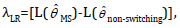, where is the MLE of parameters in the MS model and are the MLE for Θ for non-switching model, respectively. Under the null hypothesis, λ_LR has an asymptotic χ_k² distribution with k degrees of freedom, where k is the number of parameters identified under the null hypothesis. As shown in Table 3, the linearity of the λ_LR are rejected. Thus, there is a strong evidence of the existence of regime switching, which makes the use of regime switching regression models justified.

Table 3:Specification testing for MS models.

The effect of the price of coal, the price of natural gas, the price of oil and exchange rate uncertainty on the price of agricultural commodities are assessed using the two-state and three-state MS regression model. The two-state and three-state MS regression models were estimated by maximum likelihood estimation (MLE) method.

Table 4 reports the model selection criteria for the two-regime and three-regime MS models. According to the goodness-of-fit statistics such as AIC, BIC and logLik, the three-state MS approach is the best candidate model for modelling maize, wheat, soybeans and corn, however, the two-state MS approach is the best candidate model for modelling sunflower.

Table 4:Comparison of specification measures for selected agricultural commodities.

Table 5 shows the estimated parameters with their standard errors reported in parentheses. Almost all the parameters in the table are significant. This result confirms that the price of coal, the price of natural gas, the price of oil and exchange rate uncertainties do indeed play a vital role in agricultural commodity prices in South Africa. Moreover, the transition probabilities from regime 1 to regime 1, from regime 2 to regime 2, and from regime 3 to regime 3 are greater than 96% for all commodity prices. This indicates that it is hard to change from regime 1 to regime 2, from regime 2 to regime 3 and from regime 1 to regime 3.

Table 5:Maximum likelihood estimates for selected agricultural commodities.

The time varying probabilities of staying in regime 1 are reported in Figure 2. The volatility stays in regime 1 when the probability at time t is larger than 0.5, and the volatility switches to regime 2 if the probability at time t is smaller than 0.5. This confirms the existence of regime switching in the return series due to probabilities larger than 0.5 [22]. Model diagnostics such as fitted versus observed values plots (Figure 3) and residual plots (Figure 4) were used to check the validity of the fitted regime switching model. The observed versus fitted values plots (Figure 3) show that the estimated values are closely following the pattern of the observed values except corn. The residual plots (Figure 4) show that a distribution of points dispersed randomly about 0. There is no clear evidence of systematic variation indicating that the constant variance assumption is not violated.

The main aim of this paper has been to examine the factors contributing to fluctuation of agricultural commodity prices in South Africa [23]. The empirical results based on the MS regression model can be concluded as follows:

• the price of agricultural commodities was found to be significantly associated with the price of coal, price of natural gas, price of oil and exchange rate.

• for all agricultural commodities except sunflower, $k=3$ had and higher log-likelihood vales and lower AIC and BIC values. Thus, the three-state MS regression model outperformed the twostate MS regression model.

In conclusion, this paper provided a practical guide for modelling agricultural commodity prices by MS regression models [24]. This paper can be good as a reference when facing modelling agricultural commodity price problems.

None.

The author declares that there is no conflict of interest.

1. Pindyck RS (2001) Volatility and commodity price dynamics. Massachusetts Institute of Technology, Cambridge.
2. Engle RF (1982) Autoregressive conditional heteroscedasticity with estimates of the variance of the United Kingdom inflation. Econometrica 50: 987-1007.
3. Bollerslev T (1986) Generalized autoregressive conditional heteroscedasticity. Journal of Econometrics 31: 307-327.
4. Hamilton DJ (2005) Regime-Switching Models. Department of Economics, University of California, San Diego.
5. Hamilton DJ (1989) A new approach to the economic analysis of nonstationary time series and the business cycle. Econometrica. Journal of the Econometric Society 57(2): 357-384.
6. Hamilton DJ, Susmel R (1994) Autoregressive conditional heteroskedasticity and changes in regime. Journal of Econometrics 64(1,2): 307-333.
7. Raymond EJ, Rich WR (1997) Oil and the macroeconomy: a markov state-switching approach. Journal of Money, Credit, and Banking 29(2): 193-213.
8. Engel C (1994) Can the Markov-switching model forecast exchange rates? Journal of International Economics 36: 151-165.
9. Tadesse G, Algieri B, Kalkuhl M, Von Braun J (2014) Drivers and triggers of international food price spikes and volatility. Food Policy 47: 117-128.
10. Brown O, Crawford A, Gibson J (2008) Boom or bust: how commodity price volatility impedes poverty reduction, and what to do about it. International Institute for Sustainable Development, Manitoba, Canada.
11. Bellemare MF, Barrett CB, Just DR (2013) The welfare impacts of commodity price volatility: evidence from rural Ethiopia. American Journal of Agricultural Economics 95: 877-899.
12. FAO I, UNCTAD W (2011) Food and Agricultural Organization.
13. von Arnim R, Troster B, Staritz C, Raza W (2015) Commodity dependence and price volatility in least developed countries: A structuralist computable general equilibrium model with applications to Burkina Faso, Ethiopia and Mozambique. Austrian Foundation for Development Research, working paper 52.
14. Sarris A (2014) Food commodity price volatility and policy in light of Africa’s agricultural transformation. Paper presented at the annual GDN Conference Accra Ghana.
15. Tony Addison, Atanu Ghoshray, Michalis P Stamatogiannis (2016) Agricultural commodity price shocks and their effect on growth in Sub-Saharan Africa. Journal of Agricultural Economics 67: 47-61.
16. Wang J (2014) Modelling Ontario Agricultural Commodity Price Volatility with Mixtures of GARCH Processes. University of Guelph, Guelph, Ontario, Canada.
17. Acemoglu D, Simon Johnson, Robinson J, Thaicharoen Y (2003) Institutional causes, macroeconomic symptoms: volatility, crises and growth. Journal of monetary economics 50: 49-123.
18. Antonaci L, Demeke M, Vezzani A (2014) The challenges of managing agricultural price and production risks in sub-Saharan Africa. ESA Working Pp. 14-09.
19. Barrow S, Mbiyo P, Freemantle S, Silberman K, De Wet W, et al. (2017) Standard Bank Research Economic Outlook.
20. Luo C (2015) Stochastic correlation and portfolio optimization by multivariate Garch. University of Toronto, Canada.
21. Schwarz G (1978) Estimating the dimension of a model. Annals of Statistics 6(2): 461-464.
22. Zhang YJ, Yao T, He LY, Ripple R (2019) Volatility forecasting of crude oil market: Can the regime switching GARCH model beat the single-regime GARCH models? International Review of Economics and Finance 59: 302-317.
23. Akaike H (1974) New Look at the Statistical Model Identification. Automatic Control IEEE Transactions on 19: 716-723.
24. Rodrik D (1999) Where did all the growth go? External shocks, social conflict, and growth collapses. Journal of economic growth 4(4): 385-412.