On Modeling Murder Crimes in Nigeria

Crime prevention is one of the important roles of the police system in any country [1]. One of the components of crime prevention is crime forecasting. Police will require crime forecasting to make operational and tactical strategies in the future, as like to allocate police patrols in the right area, install CCTV in the right place and plan other operations [2]. In a strict legal definition, a crime is a violation of criminal law, which in most societies can be defined broadly as any ‘act or omission forbidden by law on pain of punishment’. The crime forecasting is an emerging approach in criminological research [3-4]. Crime forecasting is not widely practiced by police [5]. While there are numerous econometric studies of crime, one is hard-pressed to find police departments or other police organizations making regular use of forecasting for policing. From a more proactive standpoint, problem-oriented policing efforts may be enhanced by a more accurate scanning of areas with crime problems, in that one can examine both distributions of past crimes and predictions of future concentrations. The ability to predict can serve as a valuable source of knowledge for law enforcement agencies, both from tactical as well strategic perspectives [6]. Forecasting can help a police department’s performance by strategic deployment efforts and efficient investigation direction. The purpose of this paper is to examine the modeling and forecasting of murder rate using Auto Regressive Integrated Moving Average Models (ARIMA).

In this paper, we have used the Crime data on Murder Cases for past 29 years (1986 -2015). The crime data were sourced from Nigeria Information Resource Centre. We have used GRETL (Gnu Regression, Econometrics and Time-series Library) software for plotting the graphs and analysis of the data set.

Time series

Time series can be defined as collection of observations or measurements on quantitative variables made sequentially or in a uniform set of time period, usually daily, weekly, monthly, quarterly, annually, e.t.c Time series analysis comprises methods or processes that break down a series into components and explainable portions that allows trends to be identified, estimates and forecasts to be made. Basically time series analysis attempts to understand the underlying context of the data points through the use of a model to forecast future values based on known past values. Such time series models include ARIMA, GARCH, TARCH, EGARCH, FIGARCH, and CGARCH and so on but the main focus of this study is based on ARIMA model.

ARIMA (Autoregressive integrated moving average)

ARIMA model was introduced by Box and Jenkins (hence also known as Box-Jenkins model) in 1960. It is an extrapolation method for forecasting and, like any other such method, it requires only the historical time series data on the variable under forecasting. ARIMA models are the most general class of models for forecasting a time series [7-8]. Normally, the ARIMA model is represented as ARIMA(p,d,q) where p is the number of autoregressive terms, d is the number of non-seasonal differences, and q is the number of lagged forecast errors in the prediction equation. The identification of the appropriate ARIMA model for a time series begins with the process of finding integer, usually very small (e.g., 0, 1, or 2), values of p, d, and q that model the patterns in the data. When the value is 0, the element is not needed in the model. The middle element, d, also known as trend component is investigated before p and q. The goal is to determine if the process is stationary and, if not, to make it stationary before determining the values of p and q. The augmented Dickey–Fuller (ADF) test is most widely used test for checking stationarity of a series. If d = 0, the model becomes ARMA, which is linear stationary model. ARIMA (i.e. d > 0) is a linear nonstationary model [9]. If the underlying time series is non-stationary, taking the difference of the series with itself ‘d’ times makes it stationary, and then ARMA is applied onto the differenced series. A stationary process has a constant mean and variance over the time period. There are various methods available to make a time series stationary. Normally differencing techniques are used to transform a time series from a non-stationary to stationary by subtracting each datum in a series from its predecessor. If a series is stationary without any differencing it is designated as I(0), or integrated of order 0. On the other hand, a series that has stationary first differences is designated I(1), or integrated of order 1. The term ‘shock’ is used to indicate an unexpected change in the value of a variable (or error). For a stationary series a shock will gradually die away. In other words, the effect of a shock during time ‘t’ will have a smaller effect in time ‘t+1’, a still smaller effect in time ‘t+2’, etc. The lags of the differenced series appearing in the forecasting equations are called “auto-regressive” terms. The auto-regressive components represent the memory of the process for preceding observations. The value of p is the number of auto-regressive components in an ARIMA (p, d, q) model. The value of p is 0 if there is no relationship between adjacent observations. When the value of p is 1, there is a relationship between observations at lag 1 and the correlation coefficient ɸ1 is the magnitude of the relationship. When the value of p is 2, there is a relationship between observations at lag 2 and the correlation coefficient ɸ2 is the magnitude of the relationship. Thus p is the number of correlations we need to model the relationship. The lags of the forecast errors are called “moving average” terms. The moving average components represent the memory of the process for preceding random shocks. The value q indicates the number of moving average components in an ARIMA (p, d, q). When q is zero, there are no moving average components [10-12]. When q is 1, there is a relationship between the current score and the random shock at lag 1 and the correlation coefficient θ1 represents the magnitude of the relationship. When q is 2, there is a relationship between the current score and the random shock at lag 2, and the correlation coefficient θ2 represents the magnitude of the relationship. When one of the terms is zero, it’s usual to drop AR, I or MA component. For example, I(1) model is ARIMA(0,1,0), and a MA(1) model is ARIMA(0,0,1). The autocorrelation function (ACF) and partial correlation function (PACF) are very important for the definition of the internal structure of the analyzed series. The models can be identified through patterns in their autocorrelation functions (ACFs) and partial autocorrelation functions (PACFs).

Steps of ARIMA model

i. Identification of ARIMA (p,d,q) structure

ii. Estimating the coefficients of the formulation

iii. Fitting test on the estimated residuals

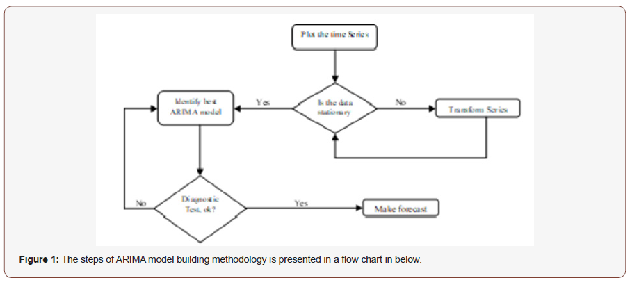
iv. Forecasting the future outcomes based on the historical data (Figure 1).

(Figure 2 & 3), (Table 1) (Figure 4 & 5)

The time series plot and correllogram of the murder data series on Figure 2 & 3 respectively shows a strong evidence of a non stationary series, the non stationarity was also confirmed with the help of the augmented dickey-fuller (ADF) test on Table 1, which tests the null hypothesis that murder data series follows a unit root process which was accepted at 5% alpha level. Implying that the murder data series is non stationary. By using first order differencing transformation, we obtained a t-statistic lesser than what was obtained at d = 0, and a p-value lesser than 5% alpha level. Thus, we select the condition that d = 1 and transform the data using first order differencing to make it stationary as seen on figure 4. The Auto Correlation Function (ACF) and Partial Auto Correlation Function (PACF) plot of the differenced series is shown in Figure 5 (Table 2).

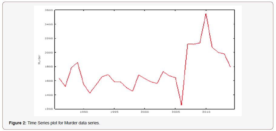
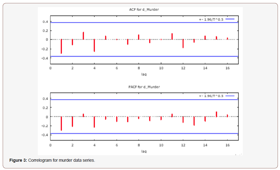
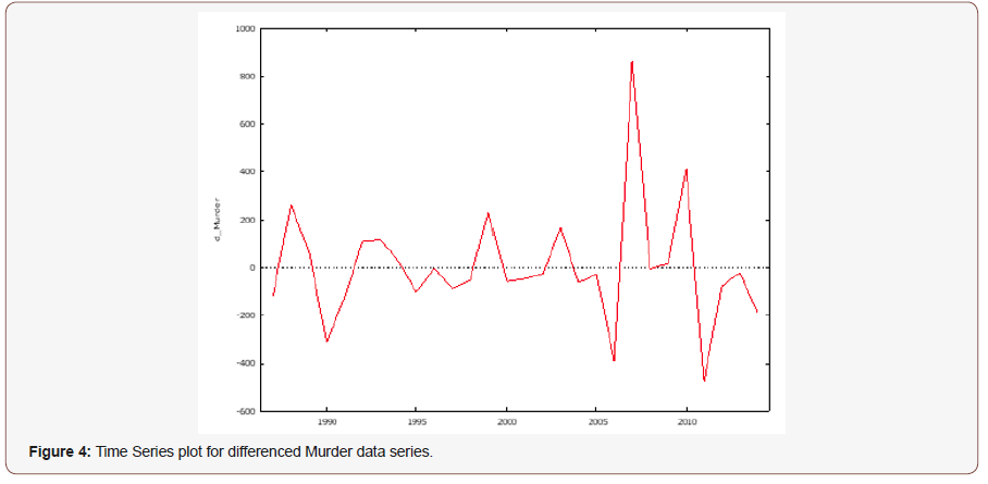
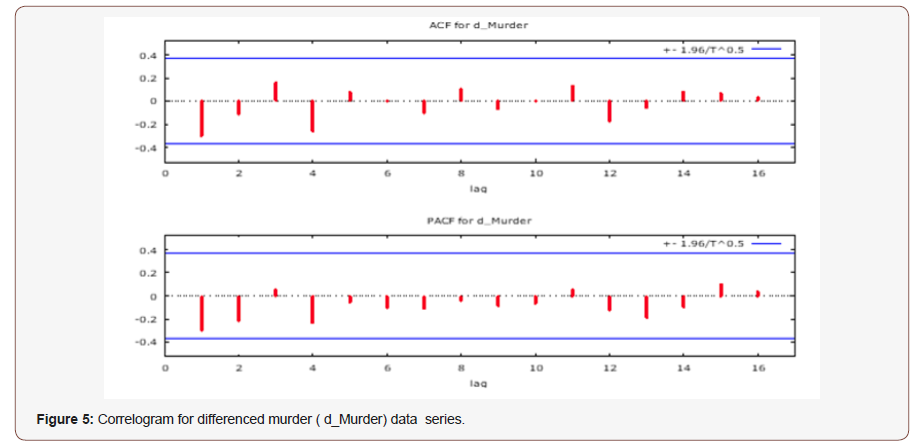
Table 1:Augmented Dickey-Fuller test for stationarity of Murder data series.

Table 2:Identification of Best ARIMA model for Murder.

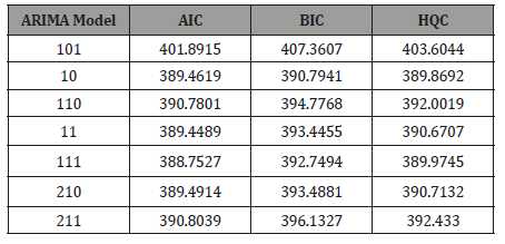
Akaike information criteria (AIC), Bayesian information criteria (BIC), and Hannan-Quinn criteria (HQC).

Seven tentative models were entertained, and the model with the minimum AIC, BIC and HQC was chosen as the best model. To verify that the chosen ARIMA (0,1,0) is an appropriate model for murder, a diagnostic check is done using residual ACF/PACF plot at different lags and testing the significance of the correlations up to 16 lags by Q statistic and respective p-values [13-14].

Diagnostic check on the best model for murder / Model verification

(Figure 6)

Figure 6 above clearly shows evidence of random walk as the values are within the bounds and undulate about zero. Hence we uphold the first order differencing (Table 3).

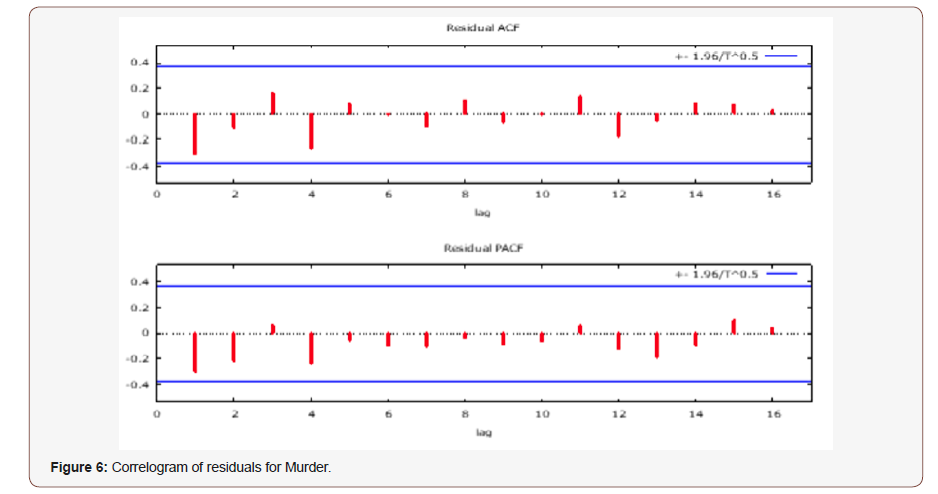
Table 3:Identification of Best ARIMA model for Murder.

Table 4:Crime Forecasting for Murder using ARIMA (0,1,0).

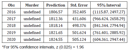
Clearly, none of these correlations is significantly different from zero at a reasonable level. The ACF and PACF of the residuals also indicate good fit of the model. This proves that the selected ARIMA model is an appropriate model (Table 4).

From the forecast on Table 4, we see that murder would increase in 2019, and in subsequent years.

ARIMA (0,1,0) has been successfully used to forecast Murder crimes in Nigeria using a twenty-nine year data series. Murder was found to be on the increase in the forecasted period. Hence, government should endeavor to sanitize the Nigerian Police Force and other security agencies. The role of the police as enshrined in the Constitution of the Federal Republic of Nigeria, as it concerns crime prevention and control cannot be over-emphasized, the development of a society largely depends on the rate of crime. If the crime rate is high, it could scare away or discourage investors. Also, the safety of lives is an issue of priority in any given society. Consequently, the government needs to increase its funding for the police so that modern and adequate equipment to combat crime could be acquired. However, such funds are to be properly monitored to avoid diversion into private pockets and also rid the Nigerian police of its corrupt elements. The family institution must also play its role by monitoring all the people in the family particularly the youth, as the police cannot fight Murder crime alone. Intelligence gathering is a veritable tool for crime prevention and control. This is why the members of the public must wake up to assist the police in its functions. The public should be ready at all times to give necessary information to the police. This is because, crime is a challenge that all and sundry must confront headlong for a stable and safe society.

None.

No conflicts of interest

1. Agyemang B (2012) Autoregressive Integrated Moving Average (ARIMA) Intervention Analysis Model for the Major Crimes in Ghana (the Case of Eastern Region), M. Sc Thesis for Masters of Philosophy in Applied Mathematics, Nkrumah University of Science and Technology Ghana.
2. Anand Kumar Shrivastav, Ekata AKS (2012) Applicability of Box Jenkins ARIMA model in crime forecasting: A case study of counterfeiting in Gujarat State. Int. J. Advance Research in Computer Engineering and Technology 1(4): 494-497.
3. Box G E, Jenkinks G M. Time series analysis: Forecasting and control. Holden Day, San Francisco, USA.
4. Bowerman BL, Connell RT, Koehler AB (2005) Forecasting Time Series and Regression: An Applied Approach. Thomson, Belmont, CA, USA.
5. Chen P, H Yuan, X Shu (2008) Forecasting crime using ARIMA model. Proceedings of the 5th International Conference on Fuzzy Systems and Knowledge Discovery 5: 627-630.
6. Gorr W, A Olligschlaeger, Y Thompson (2003) Short term forecasting of crime. Int. J. Criminol Sociol 19(4): 648-656.
7. Khashei M, M Bijari, GAR Ardali (2009) Improvement of auto-regressive integrated moving average models using fuzzy logic and Artificial Neutral Networks (ANNs). Neurocomputing 72(4): 956-967.
8. Obubu M, Nwokolo PC (2016) Modeling and Forecasting of Armed Robbery Rate in Nigeria Using Auto Regressive Integrated Moving Average (ARIMA) Models. Journal of Natural Science Research 8(6): 5-15.
9. Obubu Maxwell, Oyafajo Oyindamola Abubarkri, Anyawu Ifeyinwa Fidelia, Olayemi Joshua I (2019) “Modeling Typhoid Mortality with Box-Jenkins Autoregressive Integrated Moving Average Models”. Scholars Journal of Physics, Statistics, and Mathematics 6 (3): 29-34.
10. Maxwell O, Friday AI, Chukwudike NC, Francis Runyi E, Offorha Bright C (2019) A theoretical analysis of the odd generalized exponentiated inverse Lomax distribution. Biom Biostat Int J 8(1): 17-22.
11. Osuji GA, Obubu M, Nwosu CA (2016) “Stock Investment Decision in Nigeria; A PC Approach”. World Journal of Multidisciplinary and Contemporary Research 2(1): 1-11.
12. Osuji GA, Obubu M, Nwosu CA (2016) “Preconception sex selection using proper ovulation timing”. World Journal of Probability and Statistics Research 2(1): 1-12.
13. Osuji GA, Okoro CN, Obubu M, Obiora-Ilouno HO (2016) “Effect of Akaike Information Criterion on Model Selection in Analyzing Auto-Crash Variables.” International Journal of Sciences: Basic and Applied Research 26(1): 98-109.
14. Maxwell O, Happiness OI, Alice UC, Chinedu IU (2018) An Empirical Assessment of the Impact of Nigerian all Share Index, Market Capitalization, and Number of Equities on Gross Domestic Product. Open Journal of Statistics 8: 584-602.