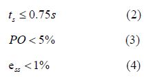
Motor Control Strategies for Drivetrain System of an Excavation Robot - Martian Surface Simulant

The design and operation of autonomous robots capable of mining Martian terrains has attracted the attention of space agencies including the National Aeronautics and Space Administration (NASA). One of NASA’s main related and inspiring projects that relates to Martian excavation is the RASSOR concept that was developed at the KSC SwampWorks center. RASSOR provides an innovative design that allows a minimization of excavation reaction forces so that optimal lightweight excavation is attainable in low gravity environments, as well as reducing launch costs [1-4]. In this work, a robot that can traverse the challenging simulated chaotic Martian terrain is intended for design and testing. The mining robot excavate the ice simulant (gravel) and return the excavated mass for deposit into the collector bin to simulate a Martian resource mining mission. The complexities include the abrasive characteristics of the regolith simulant, the weight and size limitations of the mining robot, and the ability to tele-operate it from a remote Mission Control Center. The on-site mining category requires several design and operation factors such as dust tolerance and dust projection, communications, vehicle mass, energy/power requirements, and autonomy [5].

The objective of this research is to provide an iterative process that will aid in the design and optimization of the motor control systems in a four-wheeled robot used for NASA competition. The main control objective is to obtain a smooth, responsive, and self-correcting current-controlled speed system that can be manufactured for use on future iterations of the robot. To accomplish these objectives, the process was broken into four phases –

Phase 1 – Analysis

Phase 2 – Design: Once it is established that the techniques used in Phase 1 are sufficient in modeling and analyzing the response of the generic case of a DC motor control system, the model of the motor control system of the robot will be implemented. Once the system is modeled, the parameters of current robot will be entered into the analysis techniques to develop a design for a custom motor controller that will deliver optimal performance that accounts for the robot’s weight, speed, and torque requirements.

Phase 3 – Optimization

Phase 4 – Automation [5].

This paper focuses only on the robot mobility that is provided by the drivetrain. The current progression of task fulfillment does not involve the drivetrain systems and excavation systems to operate simultaneously. The implemented strategy is first, rotate to orient, navigate to excavation site, *stop and run excavation program*, reorient to return, navigate to collector bin, *stop and run deposition program*. This article will also mainly focus on the processes used in Phase II and briefly discuss some of the future work for Phase III.

The main challenges encountered by the team are developing adequate slip-correction control strategies to implement on the current robot for effective mobility. There are well known traction models that were developed by Bekker [3] and utilized for lunar excavation purposes. However, predictive traction modeling proves to be quite difficult when operating on a surface whose soil parameters are not extensively documented. In this case, corrective control modeling is necessary. The purpose of this paper is to provide a baseline for the future RMC teams performance in competition runs, and not directly Mars exploration. It is because of this specific purpose that gravity compensation will not be considered since this robotwill only be operating on Earth. There have been proposed testing methods for excavator mobility in low gravity environments, see [4]. Figure 1 depicts the robot that this work is applied to.

All the necessary parameters were obtained to make a plant model for the DC motor (governing theory discussed in full paper [5]). Considering that the system in question requires model-based design and simulation, we chose to create Simulink block models for this system. Using the theory behind commonly used DC motor models as discussed in the Model Representation section of Phase I, along with helpful information that can be found in [7], a single-input voltage to singleoutput angular speed model for our DC motor was created as shown in the diagram in Fig. 8 of the Appendix (Figure 1).

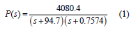
The transfer function of this model was converted into a zeropole- gain model transfer function by using MATLAB. The transfer function of the plant (our DC motors) which was utilized in all subsequent simulations is given as follows:

It is now possible to use this Simulink model of the motor to run simulations of the response for the purpose of designing a PID controller that will adequately serve the operating purposes. It is also desired to develop a repeatable process for tuning the gains of a PID controller that would work for almost any DC motor control application. Referring to the techniques established in Phase I, an uncompensated open-loop response model was created for our DC motor as shown in Fig. 9 of the Appendix, where the contents of the large DC Motor block are those displayed in Fig. 8 of the Appendix. The block on the left-hand side represents a generic step input applied at time t=0, and the block on the right-hand side represents a scope that would display the output response of the model [5]. The response of the uncompensated system is shown in Figure 2.

A. Controller Design

The primary goal of this work is to generate a repeatable method for PID controller design for systems which utilize DC motors. The first step that is necessary to begin this process is to identify which response characteristics that are desired to design around to satisfy the constraints from Phase I which are (Figure 2):

However, now that a real-world physical system is encountered, it is necessary to go through the process of defining the nominal steady-state value of the desired response for the open loop system. The physical interpretation of the uncompensated response shown in Fig. 2 states that for a 1 V step increase of the input (or, in this case, an increase in current draw from the motor that corresponds with a 1 V step increase), the response of the output angular speed of the motor shaft will increase by 56.9 rad/s [5]. It can be seen from the performance specifications for the motor that the relationship between current draw from the motor and output angular speed is linearly proportional and positively correlated. This condition also holds true for all operating points within the motor’s operating envelope. Additionally, for these systems, an increase of the magnitude of the step only significantly affects the steady-state value of the response and does not significantly affect the settling time and overshoot characteristics of the response. It is because of these system behaviors that the response behavior can accurately be predicted for larger input steps, such as the 12V operating point step, according to a unitary step response [5]. As previously determined, the output shaft angular speed at the desired operating torque is around 2400 rpm. If it is necessary for the motor shaft speed to increase 2400 rpm over a 12 V step at operating conditions, then this is the same as needing a 200 rpm increase over a 1 V step given that it has been established that the system performance constitutes linearity between current and angular speed, and therefore voltage input (again, which coincides with a change in current draw to the motor) and angular speed. It is desired to change the proportionality of the response so that every input single step increase/decrease coincides with an output increase/decrease of 200 rpm, which is approximately 21 rad/s. So, proportional control was implemented to reduce the steady state output from 56.9 rad/s to 21 rad/s [5].

The method for determining what a proportional gain value on a PID controller is described by the following relationship:

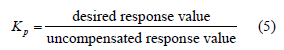
It was determined that the desired response was 21 rad/s and the uncompensated response to be 56.9 rad/s. Using this relationship, Kp was obtained to be 0.37. In order to verify the results of this proportional gain relationship, a PID controller block was added in series with the plant model in Simulink. The resulting system is shown in Figure 10 of the Appendix. Attributing a P value of 0.37 to the PID block and running the simulation, the response was obtained as shown in Figure 3.

The result in Figure 3 shows the steady-state value of the open loop response has converged to the desired output response value [5].

The takeaway steps from this portion of the controller design into the general procedure that were established can be stated as:

• Determine the desired steady-state open loop output value for a unit step that coincides linearly with the desired steady-state value at the operating step magnitude

• Tune the proportional gain to the value that caused convergence between the open loop steady-state response, with proportional control, to the desired steady-state output value (Figure 3)

Many simulations were performed at this point and the results of these simulations showed that adding derivative and integral gains to the open loop system caused undesirable results. The addition of derivative gain in the open loop system did reduce the settling time, however, never to achieve an adequate settling time. The smallest settling time achieved by adding derivative gain was about 2.2 s. In this process, it was also observed that increasing the derivative gain of an open loop system causes the overshoot of the system to increase without bound. This is highly problematic and undesirable. It was also observed that adding any sort of integral gain to the open loop system caused the response to not follow a step path but now a ramp path, which means the response increased with time and without bound. Any increase in integral gain added to the system only resulted in an increase of the slope of the ramp response [5]. To fulfill the response design criterion by implementing derivative and integral gains, it is necessary to now utilize a closed loop unity feedback system. The characteristics of unity feedback control systems have been previously discussed in Phase I and a sample figure of a closed loop unity feedback system is shown in the full report. This constitutes another takeaway step to add to the general procedure as:

• Close the loop (unity feedback) to get desired response characteristics utilizing derivative and integral gains when proportional control alone is not sufficient.

The closed loop system was modeled in Simulink to analyze the new response. A block diagram model of the Simulink closed loop system is shown in Figure 11 of the Appendix. Simply closing off the loop allows for some changes in the response time characteristics, because the system now is acting to correct an error signal. Keeping the previous proportional gain of 0.37 and running the simulation without adding derivative or integral gains, the response was obtained as shown in Figure 4. It can be seen that closing the loop without adding any additional gains does [5] (Figure 4).

Provide for a much more rapid response of the system. Where there was previous failure to achieve a settling time below the design criterion, it was now easily achieved by closing the loop without adding any additional control gain. The steady-state error, however, has increased from zero to 4.5% which will have to be rectified by introducing integral gain. Additionally, the persisting problem of an overdamped system response still exists. This can also be rectified by introducing an integral gain, as following the response characteristics [5].

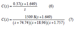
After many trial-and-error simulations, a desired “well” damped response was achieved while still fitting into the settling time requirement by implementing an integral gain of 0.61. After this tuning was performed, our final desired closed loop response was obtained which is shown in Fig. 5. It can be seen here that this response is “well” damped as it has exactly one overshooting peak above the 2% settling criterion (the two symmetrical dotted lines about 1). The overshoot is 3.89% which is less than the 5% criterion, the settling time is 0.745 s which is below the 0.75 s criterion, and the steady state error is zero. This response was obtained by using the PID gains of KP = 0.37, KI = 0.61, and KD = 0, respectively. This results in the following transfer function of the controller (in zeropole- gain format) is given as Hence, the resulting transfer function of the entire closed loop system to be (in zero-pole-gain format): (Figure 5)

The content of the final steps of the PID tuning process was combined because the derivative tuning process was evaluated and analyzed, but eventually excluded from this specific case because derivative tuning achieved undesirable results [5]. The final takeaway steps have been added to the end of the general procedure for PID tuning.

• Implement a derivative gain to the closed loop system to reduce the response time characteristics to meet the design criterion

• Readjust the derivative and integral gains iteratively, until an ID combination is found that will achieve all the required design criterion.

The control effort was plotted to verify that the requirements of the system would stay beneath the allowances of the utilized hardware [5]. The plot of the control effort for the closed loop PID system is shown in (Figure 6-10).

B. Control Strategy

The analysis and processes up until this point have only dealt with a subsystem of the RMC robot that follow the flow of operation from a single output from the microcontroller (as input to the motor controller) to the output shaft of the motor. The block diagram model of this subsystem has been previously presented in Figure 11 of the Appendix, with the step signal representing the input from the microcontroller and the scope would represent the scope connection to the two motor terminals (Figure 11).

is of importance to understand that the entire driving system involves four of these subsystems running in parallel, each receiving individual inputs from the microcontroller, as well as the gear reductions following the motor shafts and rotary encoder feedback loops to the microcontroller from each individual subsystem [5]. A block diagram of the entire robotic drivetrain control system is shown in Figure 12 of the Appendix. The previous year’s robot utilized aftermarket components (Arduino MEGA, Sabertooth 2x32) with serial data transmission to adequately perform the desired tasks of the robot. Considering that this report pertains to the mechanical performance design of a “custom” controller, this portion of control strategy will be discussed in very general terms of how the controller operates whether or not it is taking digital microcontroller input or analog input [5] (Figure 12).

The commonly used signal range to motor controllers of this size is 0 V - 5 V, whereas the main power of the motor controller, in this case, will be operating at 12 V. Since it is desired for the robot motors to operate in both forward and reverse, set up a symmetrical motor operation range about the midpoint of the signal range. This means that with an input signal of 0 V the motor will be running at full speed in reverse, and at 5 V the motor will be running at full speed forward, with the “stop” signal set at 2.5 V. A gradual increase of motor forward operation speeds will be aligned to the range of 2.5 V – 5 V of the signal, with the reverse speeds identically aligned to the range of 2.5 V – 0 V of the signal.

The actual alignment of the two sets is utilized in a simple linear conversion parameter we denote as:

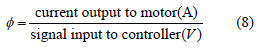
Which is essentially the slope of the linear relation. However, it is necessary to align the relationship with more than one operating point, since the signal input range is not 0 V – 5 V, but rather two symmetrical 2.5 V ranges. For this system, it is necessary to determine the actual parameters that would be utilized. The previous analysis and design sections have assumed the robot operating at full speed and fully loaded, with conservative estimations taken. It is then desired that our maximum forward/ backward current output magnitude will be the current at this operating point, 65 A. The objective is for this value to correspond to the maximum signal input of 5 V. One would encounter a slight problem when applying this to the “zero” condition versus the first forward operating point. The problem is that it is necessary for the “zero” condition to not supply any current to the motor to ensure a full stoppage. However, from the performance specifications of the motor, it is also desired that our first forward operating point to be the no-load operating current of 2.7 A. This would induce a discontinuity in the linearization if the “zero” condition was included within it. To rectify this, simply allocate two (bit) resolution ranges around the point 2.5 V to correspond with the separate “zero” condition and linearize the system beginning with the point after. For an 8-bit system, our resolution for a 2.5 V input signal range would be around 10 mV. Allocate the space from 2.49 V – 2.51 V from the signal to set the motor to the “zero” condition. Now it is possible to define that we want the no load current of 2.7 A to align with the signal voltage of 2.51V. In doing this, the linear conversion parameter was found to be 25 A/V [5].

Thus, every full Volt of signal input change should correspond to a 25 A change in current output to the motor. This also gives an incremental output resolution of 0.25 A to the motors. Given a constant torque, it has been established that an increase in current supplied to the motors will result in an increase in shaft speed from the motor. It is also known from the previously stated analysis that a change in proportional gain of the controller directly constitutes a change in the steady-state speed of the response at that input value [5].

C. Slip Correction

The slip correcting strategies in this report are based on previous work from the underlying traction model of Bekker [3]. These estimation methods are mainly used for predictive analysis and design of excavation robots for operating on lunar surface conditions. These methods may possibly also provide valid estimates for robots that would operate on Martian surface conditions as well. However, we may be able to utilize feedback control to combat slip issues without knowing these important soil parameters or gravity estimations. In other words, predictive analysis is good for design when sufficient information is present to predict how the system will perform, which is good for robotic operation on Earth, Mars, or on the Moon. However, if we utilize correction through control strategies, we could develop a system that would be able to operate adequately on any soil surface with little known or unknown soil parameters. As the purview of space exploration grows, this concept will be extremely important for future celestial body exploration [5].

We will look at control strategies that involve accounting and correcting for slip. Slip is defined as

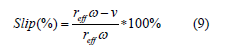
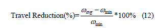
Where v is the vehicles linear velocity, 𝑟𝑒𝑓𝑓 is the effective wheel radius, and ω is the angular velocity of the wheel shaft. The effective radius is an equivalent radius where shear occurs between moving soil and static soil. The estimation of the effective wheel radius does not have a well-known consensus and does not have properly defined precedent. Because of this, another parameter known as travel reduction is used instead of slip

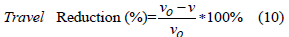
Where 𝑣𝑜 would be the vehicles baseline speed on flat ground with no drawbar load applied. The work done by Skonieczny [4] implies that it is of utmost importance to keep the drawbar pull (normalized by weight) ratio below about 0.24 for lightweight excavators. At this point, excavator performance crosses a “lightweight threshold” where travel reduction spikes from 20% to 80% [5].

The strategy to combat slip is based on the concept of travel reduction through using sensors on the robot. The robot will continue to perform well if the travel reduction is held below 20%. We can apply rotary encoders to the wheel shafts to keep a constant measurement of the wheel shaft angular velocity to be sent back to the motor controller. If applying an encoder to each of the four shafts, we can estimate that our baseline speed on flat ground is

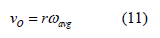
Where avg ω is the average encoder measurement of the motor shaft speeds at a given instant [5]. The author currently is considering two different methods of using sensors to determine the actual linear speed 𝑣. We have proposed a method which utilizes the rotary encoders of the system to determine the travel reduction and correct for slip. The method proposed is as follows:

It is a common simple practice to estimate traction through shaft speed as though the actual speed of the robot corresponds with the minimum measured shaft speed of the wheels. That is, the slowest moving wheel is the one which has traction and therefore that speed corresponds to the vehicle’s propulsion speed. The measurements could be directly fed back to the microcontroller and computer to run through a program and compute a value for travel reduction as

Then, the strategy taken to combat this slip would be to amplify the proportional gain on the controller, to supply more power to the motors, that corresponds 80% of the current experienced travel reduction. The new proportional gain value to be used would come from

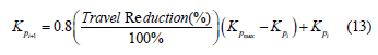
Where the subscript i is the uncompensated, subscript max is the maximum operating condition as previously discussed, and subscript i+1 is the adjusted value [5].

The primary objective of this portion of the work was to obtain a rapid yet smooth response of the RMC motor control system by utilizing the established control tuning strategy. The overlaying objective is to verify that this control tuning strategy will prove to be a consistent and effective way of determining PID gains for a variety of different DC motor applications. This objective is a work in progress, and the utilization of this strategy upon many more systems to verify its effectiveness. A proposed testing method which we wish to perform in the coming year is to build a practice run pit so that the actual number of excavation trips per 10-minute run that can be performed by the robot can be determined. This would greatly help the team in more rapidly determining what areas of the robot need to be optimized to achieve better competition performance [5].

None.

No Conflict of interest.

1. L Parrish (2013) “Regolith Advanced Surface Systems Operations Robot (RASSOR) Excavator,” NASA Technology Transfer Program, pp. 1-2.
2. Heiney A (2018) NASA’s Ninth Annual Robotic Mining Competition: Rules and Rubrics. Retrieved May 10, 2018, https://www.nasa.gov/sites/default/files/atoms/files /2018_rules_rubrics_parti.pdf
3. Bekker M (1969) Introduction to terrain-vehicle systems. University of Michigan Press. Ann Arbor, MI.
4. Skonieczny K (2013) Lightweight Robotic Excavation. Carnegie Mellon University: 51-71.
5. Crawford (2019) “Motor Control Systems Analysis, Design, and Optimization Strategies for NASA RMC Excavation Robot,” MS Thesis, University of Arkansas.
6. Bishop RH, Dorf RC (2011) Modern Control Systems (12th ed.). Upper Saddle River, NJ: Pearson Education.
7. (2021) DC Motor Speed:  Simulink Modeling. (n.d.). Retrieved May 12, 2021, http://ctms.engin.umich.edu/CTMS/index.php?exa mple=MotorSpeed&section=SimulinkModeling