Enabling a Mobile Robot for Autonomous RFID-Based Inventory by Multilayer Mapping and ACO-Enhanced Path Planning

Keeping accurate inventory is crucial for the retail industry to stay profitable and efficient. Traditionally, most retail stores perform manual inventories that are costly, inefficient and error prone. Since the last decade, radio-frequency identification (RFID) technology has been widely adopted by retailers [1]. However, even equipped with RFID technology, existing tools and systems still rely on employees to carry readers to scan the tag of each product. Employees move around and make their own decisions while scanning. To increase inventory efficiency and reduce labor cost, retailers have attempted to deploy autonomous mobile robots for RFID-based inventory [2-5].

In this paper, we introduce a systematic approach that enables robots with onboard RFID-readers to autonomously perform accurate inventories for retailers. Retail environments are dynamic and complex. To safely and efficiently perform inventory counts, robots must be able to navigate without colliding with obstacles. To overcome this challenge, an algorithm for building a high-quality map that can precisely represent the surrounding environment is necessary. A common method that allows a robot to build a map in an unknown space is known as simultaneous localization and mapping (SLAM) [6].

For indoor robotic applications, light detection and ranging (LIDAR) sensors and stereo or RGB-D cameras are the most widely used mapping sensors. However, mapping methods using a single sensor have obvious limitations. First, LIDAR sensors scan the environment, detect objects on a 2D plane, and then provide precise relative distances and angles of each item. However, the 2D map built by LIDAR is unable to describe the complicated geometric features of an object-rich, confined retail environment. Alternatively, stereo or RGB-D cameras simultaneously collect depth and RGB information and images. Then, each pixel of the RGB images is paired with the corresponding depth value of the depth image. Subsequently, 3D point clouds are generated to reconstruct the surrounding environment. However, due to limited field of view (FOV) of the camera, robots lack the ability to obtain reliable and accurate pose estimation.

In addition to accurate mapping, RFID-enabled robots work quickly and consume little power, therefore reducing operational time and resource consumption. Inventory can be performed more frequently and dynamic changes in stock can be precisely recorded. Additionally, these robots move close to shelves stocked with RFIDtagged products and scan all tags until the entire target space is covered. When finished, they return to the initial launch point. To decrease the time-cost of inventory counts, the robot requires an optimized path with the shortest navigational distance throughout the whole inventory route. The challenge of ensuring the robot visits all locations of interest without repeating is known as a typical Traveling Salesman Problem (TSP). There has been some pilot work utilizing various algorithms, such as the Genetic Algorithm (GA) for the TSP, to optimize the path of mobile robots [7].

In this paper, we propose a novel approach that provides precise maps and optimizes the inventory path in a retail environment. For mapping, a new method-called multilayer mapping-fuses the LIDAR and a Microsoft Kinect RGBD camera (hereafter, Kinect for short) to create a precise and feature-rich map of the surrounding environment. It relies on LIDAR to provide frequent and reliable poses of the robot, while Kinect offers abundant details of the complicated environment for map building. The map generated by this multilayer mapping method contains precise poses and abundant structural features of the surrounding environment. Hence, it can accurately reconstruct the complex environment and support effective inventory operations. Motivated by the method introduced in [3], the robot is equipped to scan RFID tags in a target space by following a designated path determined by the unique requirements of the employed RFID technology and created map. The Ant Colony Optimization (ACO) algorithm is implemented to minimize the total distance of the inventory route without affecting inventory accuracy. The main contributions of this paper are as follows:

1) Develop a method that fuses a LIDAR sensor and an RGB-D camera to precisely map complex indoor environments, such as retail stores.

2) Implement the ACO algorithm to optimize an inventory path that minimizes the whole navigational distance while maintaining inventory accuracy.

3) Create a prototype system and conduct several experiments in a mock apparel store. Results demonstrate that our proposed method can efficiently and autonomously execute RFID-based inventory and provide accurate inventory outputs.

Deploying a robot in a retail environment is not a new idea; recently, several pilot projects have explored this topic [8-12]. Additionally, some robotic applications have been adopted for customer assistance, inventory control, and other uses in retail stores, distribution centers, and warehouses. However, it is a challenge to deploy autonomous robots in a complex retail environment. Doing so requires careful attention to environment mapping, navigation strategies, and sensor technology.

Pilot initiatives of retail automation applications

A robot assistant that directly interacted with customers was designed by Brodeur [13]. Agnihotram introduced a robot to patrol the store and provide autonomous shelf analysis to track dynamic product stocks in retail [14]. Based on machine learning algorithms, the robot was trained with selected parameters to detect product boxes with computer vision technologies. Meanwhile, RFID technologies are widely deployed for a similar concept. Melià-Seguí conducted an RFID-based installation in a clothing shop in Barcelona [15]. The application interacted with customers for several months. Massimo designed an RFID gate for fashion retailers [16], and experiments were performed to test the efficiency of the gate’s RFID tag reading process. Motroni presented the phase-based SARFID algorithm to locate static RFID tags with UHF-RFID readers [17].

In addition to these initial trials of deploying automated RFID technology in the retail industry, increasingly more research has focused on combining RFID and robots. Ehrenberg designed the LiBot system for autonomous library book checking [18]. The LiBot system enabled the robot to read shelves and locate misplaced books. Product stock in retail must be recorded routinely, and object counting is commonly used for inventory management. Schairer introduced an RFID-based, machine-supported inventory system [19]. A robot with an RFID reader continuously detected RFID-tagged products in a simulated supermarket environment. Miller combined LIDAR and RFID readers on a robot platform to design the Automated Asset Locating System (AALS) [20]. A robot with AALS was able to autonomously detect more than 100 target tags along a 1.4 km navigation path.

Mapping methods

One of the most critical tasks for an autonomous mobile robotic system is to precisely map the surrounding environment. Introduced by Durrant-Whyte, SLAM is a fundamental function in mobile robotic research and applications [21]. There are several SLAM methods, including the extended Kalman filter (EKF) using SLAM and FastSLAM using the Rao-Blackwellized filter [22,23]. SLAM implementations are classified according to the sensors mounted on the robot. For this research, we focused on LIDARbased SLAM, visual SLAM, and sensor fusion SLAM.

LIDAR-based SLAM methods have been widely used in previous decades. LIDAR extracts discrete points that describe distance and orientation of objects [24]. The nature of LIDAR guarantees highly accurate object detection, and, hence, generates high quality maps. Additionally, optical density has no impact on LIDAR, so LIDARbased SLAM methods can be performed in both indoor and outdoor environments [25, 26]. Alternatively, visual SLAM methods generate 3D maps with rich environmental information using stereo, RGB-D, or monocular cameras. Paz presented stereo SLAM in the early years [27]. R.A. Newcombe developed RGB-D SLAM based on Kinect [28]. Engel performed LSD-SLAM to build a large-scale map using a monocular camera [29]. More visual SLAM approaches, including RTAB, and ORB-SLAM, have been developed in recent years [30,31].

However, the maps generated by low-cost 2D LIDAR lack vertical information to describe complicated environments. Additionally, visual SLAM approaches obtain poor pose estimations when locating the object coordinates or a robot in space. To overcome these issues, sensor fusion methods for mapping are developed by merging information from both LIDAR and Kinect [32]. However, information loss occurs during the merging process. In our paper, we introduce a multilayer mapping approach that reduces information loss.

Robotic navigation approaches

Path planning strategies for robot navigation can be classified as local and global. Local path planning prioritizes motion control and collision avoidance, while the global path planning prioritizes generating routes for robots so that they may to complete navigation [33-35]. We focus on the global path planning algorithms for this paper. The A-star (A*) algorithm was first published in 1968 and is widely used for robot path planning [36,13]. Later, the probabilistic roadmap (PRM) planner was introduced based on the A* algorithm to improve its efficiency [37,38]. Although the A* algorithm and PRM are widely applied to ground robots, the Rapidly-Exploring Random Tree (RRT) is utilized for aerial robots and robotic arms [39, 40].

The RRT generates global paths for robots that require high dimensional motion. Different from the robot’s task of only moving from a starting point to a target, the inventory task in our paper requires the robot to return to the starting point after visiting multiple targets. Global path generation is, therefore, the same as the TSP. Various optimization algorithms, including the Genetic Algorithm (GA), Simulated Annealing (SA) and Ant Colony Optimization (ACO) are widely implemented for TSP optimization [41-43]. According to the comparison of experiments from [44,45], ACO provides the best optimization results for medium and largescale TSP, which includes more than 50 vertices. Therefore, we select the ACO method to generate global paths, which comprise a larger number of discrete destinations, for robots monitoring inventory in retail environments.

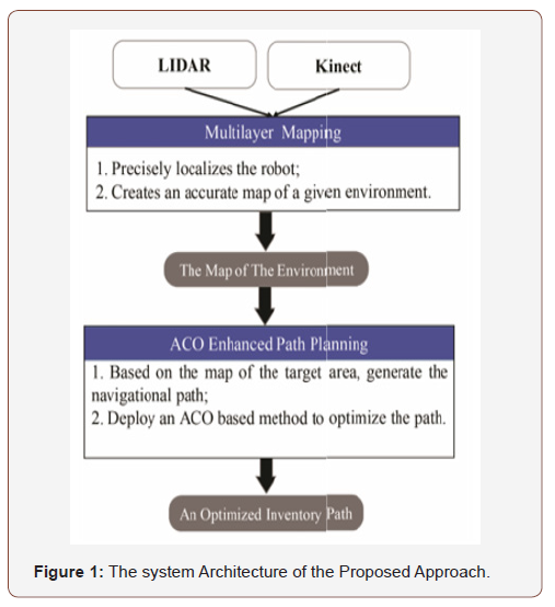
Our proposed method consists of two components, multilayer mapping and ACO-enhanced path planning. Multilayer mapping creates a reliable map that enables subsequent ACO-enhanced path planning to navigate the robot throughout a complex indoor environment for efficient inventory counting (Figure 1) illustrates the architecture of our proposed method.

Multilayer mapping

Creating a map for a robot in an unknown area can be accomplished using the SLAM approach [21]. The nature of traditional SLAM relies heavily on the accuracy of observation. Our proposed multilayer mapping method fuses LIDAR and Kinect information together. This method receives pose estimation information from LIDAR and rich environmental information from Kinect to generate a map. The precise poses of the robot and substantial feature details from RGB-D images guarantee the generated map can reliably and accurately represent a complex environment.

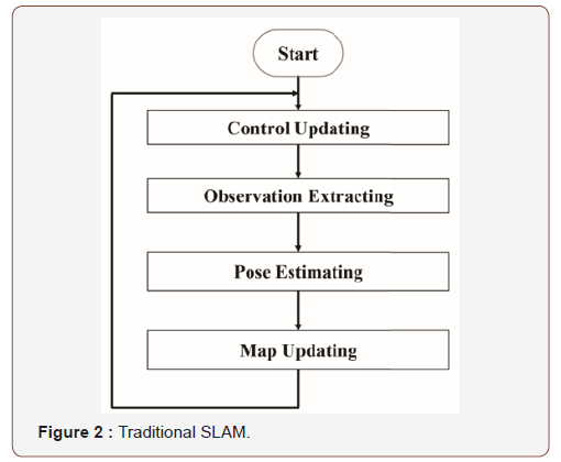
SLAM: As shown in (Figure 2), traditional SLAM process builds a map by the iterative process of control updating, observation extracting, pose estimating, and map updating [21]. Based on the control commands, SLAM predicts the position and heading of the robot against its previous pose. SLAM then receives observation data from LIDAR, camera or sonar sensors. Together with the observation data and the predicted pose, SLAM estimates the current pose of the robot. Lastly, SLAM updates the map with the robot’s current pose and observation data. It continues this cycle until the map building process is complete. As one of the fundamental functions of the mobile robot, there are various implementations of SLAM, and Rao Blackwell Particle Filter (RBPF) is widely used for robot tracking [46]. The core procedure of the traditional RBPF based SLAM can be represented by the following equation:

Here, x presents the pose of the robot, 𝑚 is the map, 𝑧 denotes the observation from sensor, and 𝑢 refers to the control command (e.g. the odometry information).

estimates the pose of the robot based on the control commands and observations. It is a typical localization problem in the robotics community, and there are many solutions available, including the Monte Carlo localization algorithm [47] that provides robust pose estimation.

updates the map based on the given pose of the robot.

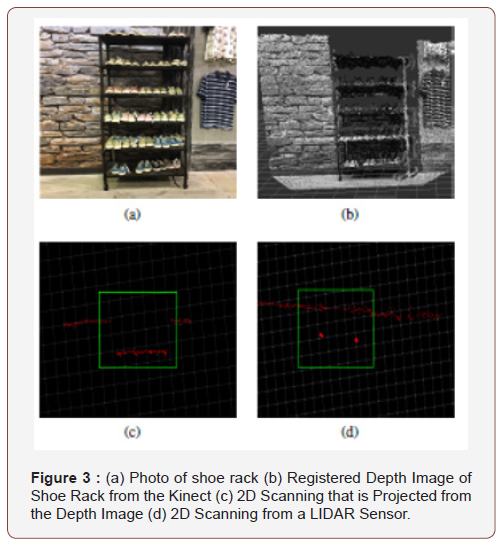
The process of multilayer mapping: Equation (1) shows that the observations from a sensor are critical for the SLAM process. However, use of a single sensor hinders robust and reliable implementation of traditional SLAM. Therefore, we conducted a benchmark experiment to overcome this challenge. In this experiment, a 360 degree Lase Scanner Development Kit (RPLIDAR) [48] and a Microsoft Kinect were selected. The RPLIDAR only provides a 2D slice of the surrounding environment. Although existing obstacles outside of the scanning plane of RPLIDAR could cause a collision during navigation, its longer sense range and wider angle of FOV provide precise pose during the SLAM process. Alternatively, Kinect captures 3D images that contain tremendous detail of the environment in a smaller FOV. We compared the output of those sensors in (Figure 3,3a) is a photo of a shoe rack and (Figure 3b) is the corresponding 3D image generated by Kinect. It is obvious that the 3D image shows much more structural information about the shoe rack. Usually, the 3D image would be converted to 2D scan data due to inadequate computing capability of cost-constrained indoor robots [49]. (Figure 3c) illustrates the 2D scan data projected from Kinect’s depth image, and (Figure 3d) shows the 2D scan data from RPLIDAR. Here, the red dots represent the edges of detected objects in the surrounding environment. Obviously, the observations of LIDAR alone cannot correctly detect the shoe rack. RPLIDAR only detected the columns of the rack that were presented as several dots in the scanning output. RPLIDAR supports a much wider FOV that enables it to detect more objects from the surrounding environment, whereas Kinect has a limited FOV (about 57 ⁰ horizontally and 43 ⁰ vertically) that can only detect the front of the shoe rack. Thus, a short sense range and narrow FOV prevent Kinect from estimating a precise robot pose.

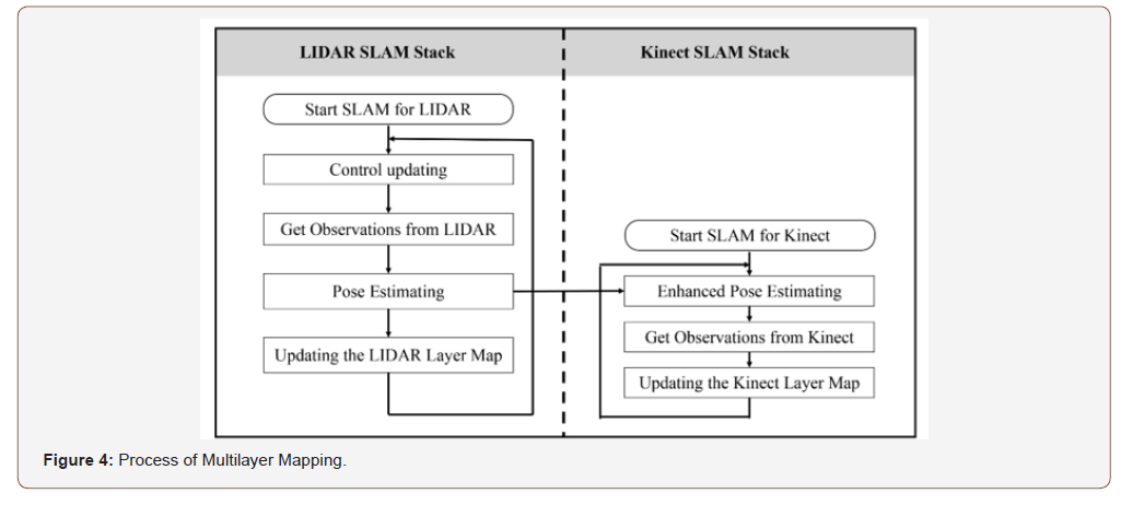
It is necessary to integrate data obtained from both LIDAR and Kinect when using both types of sensors [50]. First, we synchronized observations from the different sensors. For example, Kinect provides observations in 30 Hz while the frequency of most LIDAR updating is less than 10 Hz. Second, we addressed the issue of information loss that occurs during the merging process. LIDAR only scans a 2D plane and obstacles out of its limited scanning plane are missed. Therefore, SLAM may treat the objects detected by Kinect as noise or temporary obstacles and refuse to update the map. Hence, it is difficult to generate a consistent map during merging. To overcome the limitations of using single sensor in map building, we created a multilayer mapping method in which both LIDAR and Kinect are deployed to offer sufficient observation information and compensate each other. Instead of merging the observations from multiple sensors for a single SLAM stack, we start one SLAM stack for each sensor. The process of multilayer mapping is shown in (Figure 4). In our proposed method, the two SLAM stacks work together to produce a multilayer map. The LIDAR SLAM stack generates a reliable pose estimation of the robot, which enhances the inaccurate pose estimating of the Kinect SLAM stack. In this way, two separate map layers with high consistency in coordinates are obtained to form a multilayer map. From this map, we obtain accurate poses and all useful structural information of the environment.

As shown in (Figure 4), the LIDAR SLAM stack is the same as a traditional SLAM process with control commands and LIDAR information as its inputs. In this process, the pose of the robot is estimated, and a LIDAR-layer map is generated by the observations from LIDAR. Another process, the Kinect SLAM stack, is based on the poses from LIDAR SLAM stack to enhance its pose estimation. Instead of estimating pose from the observations of Kinect and control information, the Kinect SLAM stack gains the pose from the LIDAR SLAM stack and control command updates (otherwise known as Enhanced Pose Estimating). The concept of Enhance Pose Estimating is shown by the following equations:

Here, t' x denotes the latest (at time 𝑡′) estimated pose from the LIDAR SLAM stack, 𝑢_Δ𝑡 represents the updated control commands in time period Δ𝑡 (Δ𝑡 = 𝑡 − 𝑡′). Function 𝑓(.) updates the pose according the control commands. Since t' x is a precise pose estimation, Δ𝑡 is a very short time period between LIDAR and Kinect observations. The estimation of pose 𝑥𝑡 contains very little error that is introduced by the control update, and that is precise enough for our mapping. The update of Equation (1) for the Kinect SLAM stack is:

By registering the RGB-D observations from Kinect along with enhanced pose 𝑥𝑡, the Kinect layer map shows highly precise environmental features. Furthermore, because 𝑥𝑡 is updated by t' x , the LIDAR layer map and the Kinect layer map are very consistent. Therefore, with precise poses and abundant details provided by the multilayer map, the effective performance of robot navigation is guaranteed.

ACO-enhanced path planning

For an RFID-equipped robot to conduct autonomous inventory counts in a retail environment, path planning must consider the requirements of RFID technology. Meanwhile, to improve the performance of inventory counts, the robot must read all RFID tags in a target space while reducing total moving distance. Consequently, ACO-enhanced path planning can fulfill those requirements [51].

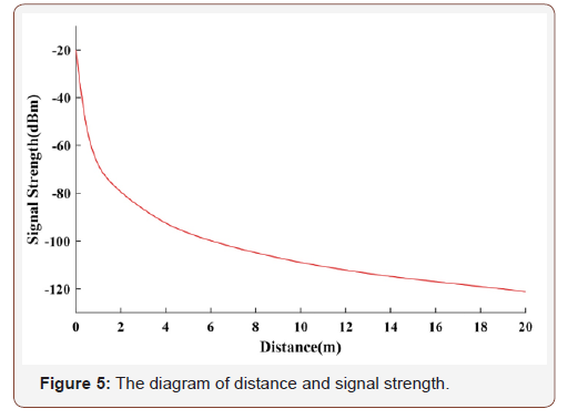
The UHF-passive RFID sensor model: Due to its low-cost and capacity to offer unique identification of individual items, ultra-high frequency (UHF) passive RFID technology is widely deployed in the retail industry. In a passive UHF RFID system, when a tag receives a continuous wave (CW) from the reader, it absorbs the energy and backscatters CW to communicate with the reader [52]. The signal strength attenuates dramatically while the distance between the reader and tag increases. A typical relationship between distance and signal strength is shown in (Figure 5) [51]. Therefore, a reader can only detect the tags in a limited range (e.g., most commercial off-the-shelf UHF RFID readers can only read tags within several meters). Furthermore, this range is greatly reduced by the objects and structures that occur in an indoor environment. When a tag is out of the detectable range of the reader, detection failures occur.

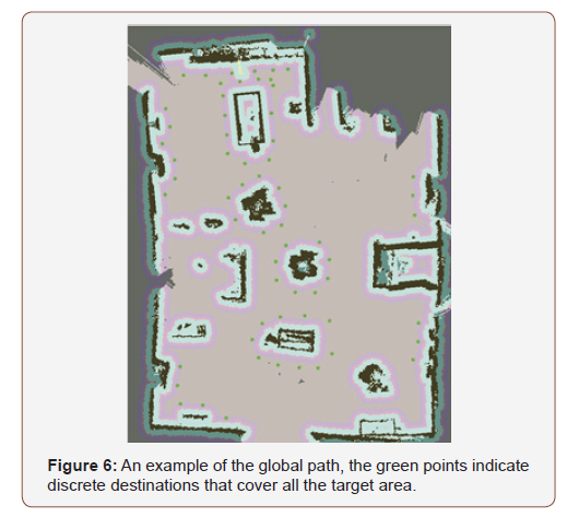
Inventory path design: Motivated by the path planner introduced in paper [3], a navigational path can be generated from the map created by our multilayer mapping method. This path can guide the robot to autonomously perform inventory counts. Here, the path planner consists of a global and a local path planner. The global path planner generates the inventory path to pilot the robot while counting inventory. It considers requirements of the UHFpassive RFID sensor model to guide the robot as it navigates close to merchandise to scan for RFID tags. It provides a group of discrete goals to represent the path. When the robot navigates to all of the goals, it will have completed an inventory count within the target space. (Figure 6) illustrates an example of a global path. The local path planner focuses on how to safely navigate the robot between goals in the global path, we chose the Dynamic Window Approach (DWA) method as our local path planner to navigate without collision [53].

Traveling salesman problem: The global path is a set of discrete destinations such as those shown in (Figure 6). The robot needs to visit them all to carry out inventory counting. To improve inventory Efficiency, the robot needs to arrive at all destinations without moving back and forth so it can maintain minimal total traveling distance [54]. Usually, the robot needs to return to the same place where it started. This process is exactly the same as the TSP. As the name TSP implies, a salesman needs to travel to all the cities on a list without repeating a visit and return to the departure city. It needs to select the shortest route that contains every city. Along the graph of the route, cities are referred to as vertices or points, and we will use the terms of city, point, and vertex changeably hereafter. We assume that there are 𝑛 total points in a global path During an inventory, the cost for the robot move between two points is unrelated to the visiting direction.

edge. The optimization of the TSP is to select the edges that connect all vertices in a closed loop with the minimal total weights [55].

Aco-enhanced path planning: We deploy the ACO algorithm to solve the aforementioned TSP and provide an optimized navigational path for the robot to perform an RFID inventory autonomously and efficiently. ACO is inspired by the natural behavior of an ant colony [56]. A group of ants tend to find the shortest path to the location of food and return to the colony. A single ant can only behave simply, however, a group of ants is able to accomplish tasks with high complexity. Ants leave the colony and randomly choose a path to the location of food. When an ant travels, it leaves pheromone signals on the path. The pheromone evaporates as time passes. Along a shorter path, it takes less time for an ant to find food and return to the colony. Hence, during that same time period, any amount of pheromone left along on the shorter path will be more than that left on a longer path, as ants tend to select the paths with more pheromone according to biological instinct. Gradually, the selection of shorter paths converges until only one short path remains [43].

ACO is widely used for optimizing various problems, as it tends to find global optimizing results rather than being trapped into local optimization [57]. Usually, the ACO algorithm is implemented in an iterative manner and there are two steps within it in a typical iteration updating. The first step consists of the state transition between each point the ant chooses next. When an ant 𝑘 is about to move to the next point, it makes the decision by following pseudorandom proportional rules [58].

In (4), 𝑠 represents the next vertex 𝑣𝑗 that ants move to. τ (i, j) stands for the amount of pheromone left on path 𝑒𝑖𝑗. η (i, j) is the heuristic function that estimates the fitness of the path. In ACO, the value of η (i, j) is the inverse of weight 𝑑𝑖𝑗. 𝛽 decide the weights of η (i, j) . All unvisited vertices are evaluated using Equation (4). The number 𝑞 is chosen randomly from the range [0,1]. 𝑞 0 is the threshold that decides whether to perform probability searching or not. If 𝑞 is less than 𝑞0, the ant selects the vertex with the maximum value as its destination. Otherwise, 𝑆 is generated following the probability distribution in Equation (5). Formula (5) represents the probability of the vertex, 𝑣𝑗, that would be chosen as the destination by ant 𝑘 at current vertex 𝑣𝑖. P_k (i ,j ) i j represents the probability distribution of the ant k at current vertex 𝑖 moves to a selected vertex 𝑗. 𝑆 denotes the selected vertex 𝑗 that is generated randomly following the probability distribution P_k (i ,j ) i j . The notation 𝐽𝑘(𝑖) is the list that contains the unvisited vertices of ant 𝑘 at current vertex 𝑣𝑖.

The second step consists of the rules for pheromone signals along the paths on the map. As time passes, the previous pheromone signal evaporates while ants come and leave new signal on the path. Pheromone signal updating follows Equations (6) and (7). In Formula (6), τ (i, j) stands for the amount of pheromone left on the path 𝑒𝑖𝑗, and 𝛼 denotes the weight of the remaining pheromone from the previous iteration. 𝑁 is the number of ants in the ACO. 1

distance 𝐿𝑒𝑛𝑔𝑡ℎ𝑘 of the trip completed by ant 𝑘. When ant 𝑘 has visited all vertices, it is regarded as that the ant 𝑘 finished the tour. Then, the distance of the tour cycle is computed.

Destination selection and pheromone signal updating construct the ACO iteration. The optimal path is gradually generated in iterations of ACO (Figure 7) shows the process of ACO.

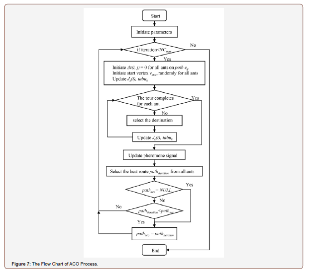
At the initiating step, the maximum iteration, 𝑁𝐶_𝑚𝑎𝑥, is set. When the iteration grows larger than 𝑁𝐶_𝑚𝑎𝑥, ACO finishes. The vertices with coordinate information are sent to ACO as preparation. The distance between vertices is calculated and 𝜂 (𝑖, 𝑗) for each path is generated. The number of ants is configured. Using a large number of ants in ACO will reduce the number of iterations needed for convergence but increase the time cost of each iteration. To keep a balance of convergence and the time cost of each iteration, we set the number of ants similar to the quantity of vertices. Following the suggestion in paper [59], we set 𝛽 to 4 and 𝛼 to 0.9. Additionally, we set 𝑞0 to 0.2 to rely more on probability searching. Before starting the ACO iteration, the pheromone distribution on each path was kept the same. The parameter τ (i, j) for all path was initiated to 1. We built a group of empty lists, 𝑡𝑎𝑏𝑢, to record the visiting sequence of all ants. In our paper, the optimal output of ACO is the inventory route with the minimum total distance. The best route is set as 𝑝𝑎𝑡ℎ_𝑎𝑐𝑜 to store the total distance and visiting sequence. Before the iteration, 𝑝𝑎𝑡ℎ_𝑎𝑐𝑜 is set as 𝑁𝑈𝐿𝐿.

At the beginning of each iteration, the start vertex 𝑣𝑠𝑡𝑎𝑟𝑡 is randomly generated for each ant, 𝐽_𝑘(𝑖) is updated by deleting the last visited vertex, and 𝑡𝑎𝑏𝑢𝑘 records the current location of ant 𝑘. If there are vertices remaining on the list 𝐽_𝑘(𝑖), ant 𝑘 selects the next vertex as the destination following Equations (4) and (5). Otherwise, the tour of ant 𝑘 is complete. During the ACO iteration, 𝐽_𝑘(𝑖) and 𝑡𝑎𝑏𝑢𝑘 continuous update the status of tour completion along the trajectory of ant 𝑘. After all of the ants finish their tours, the pheromone signal left on the path updates according to Equations (6) and (7). During each iteration, the distance of the route that is completed by each ant is calculated, and the best route 𝑝𝑎𝑡ℎ𝑖𝑡𝑒𝑟𝑎𝑡𝑖𝑜𝑛 with the minimum distance is determined. The 𝑝𝑎𝑡ℎ𝑎𝑐𝑜 is updated based on the current 𝑝𝑎𝑡ℎ_{𝑖𝑡𝑒𝑟𝑎𝑡𝑖𝑜𝑛}. The 𝑝𝑎𝑡ℎ𝑎𝑐𝑜 only stores the shortest 𝑝𝑎𝑡ℎ_{𝑖𝑡𝑒𝑟𝑎𝑡𝑖𝑜𝑛} among all executed iterations. Hence, after the number of iterations times reaches 𝑁𝐶_𝑚𝑎𝑥,𝑝𝑎𝑡ℎ_𝑎𝑐𝑜 provides an optimal route result that includes the shortest distance and visiting sequence. Usually, 𝑁𝐶_𝑚𝑎𝑥 is selected empirically, it is configured as 150 in all our experiments.

Experimental setup

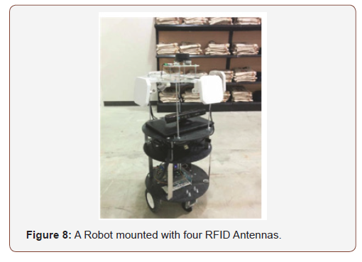
Robotic platform: The REX-16D Round Robot Base from Zagro Robotics was chosen for the hardware platform of our robot. It is equipped with two driver motors and two caster wheels that support 360-degree rotation. Three 14-inch ABS plastic boards make up the chassis of the robot, which hosts the on-board controller, sensors, and batteries. An additional disk was installed on the chassis to mount the RFID antennas. For our robot’s sensors, we choose a Microsoft Kinect and a RPLIDAR 360-degree laser scanner to obtain data for map building and robot navigation. We selected the Zebra FX9500 to read RFID tags and placed four Zebra AN720 antennas on the robot for inventorying. The photo of our prototype robot platform is provided in (Figure 8).

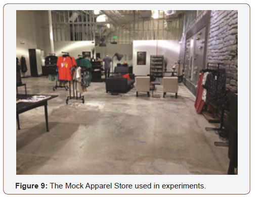
Experimental results

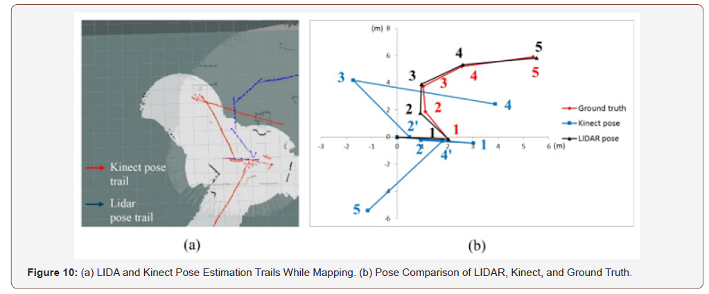
Assessment of multilayer mapping: We conducted experiments to evaluate the performance of multilayer mapping in a retail context. A map of the mock store was created from scratch, and, during the mapping process, the robot was manually piloted by keyboard commands to explore the entire store. (Figure 10a) is a screenshot of running standard SLAM on Robot Operating System (ROS). (Figure 10b) shows the sampling points of pose estimation trails of (Figure 10a) in sequence. As previously mentioned, the Kinect cannot provide an accurate pose due to its limited observation ability, while LIDAR can provide relatively accurate pose estimation because of improved FOV. According to (Figure 10b), when the robot changes directions, the pose estimated by LIDAR data is precise, whereas Kinect’s pose estimate is prone to larger error. This is because when the robot turns around, observation data change dramatically. In such cases, it is difficult for Kinect SLAM to match the correct parts in the map, which results in significant errors of the estimated poses, as shown in (Figure 10b) at point 2 (2’) and point 4 (4’) of the Kinect pose trail. Here, point 2’ and Point 4’ denote the estimated positions when the robot suddenly changes direction (at point 2 and point 4, respectively). Additionally, we compared the localization accuracy of LIDAR SLAM and Kinect SLAM in (Table 1). This table shows that for LIDAR, smaller errors are made during turns and the errors can be controlled within a certain range thanks to FOV.

Table 1: Pose Estimation Errors of LIDAR and Kinect lingerie table.

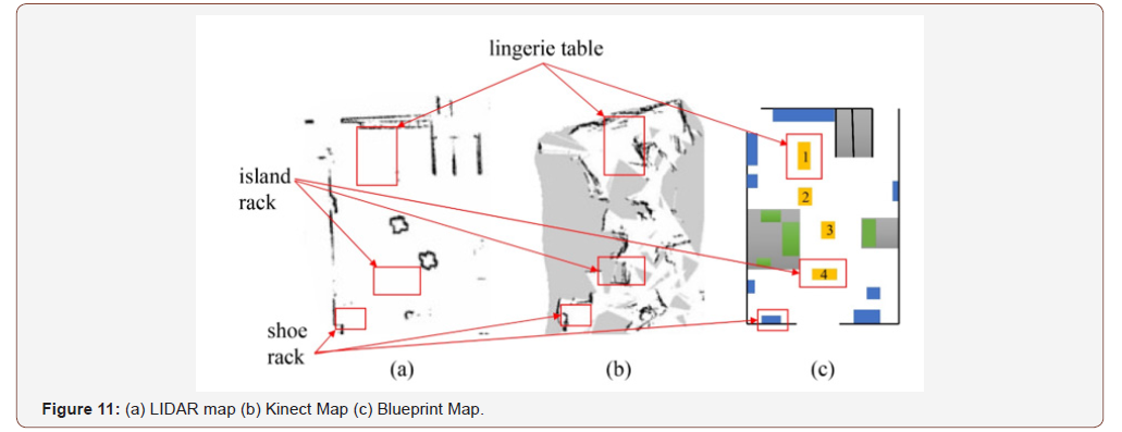
(Figure 11) shows the maps generated by SLAM with LIDAR (LIDAR-map, Figure 11a) and by SLAM with Kinect (Kinect-map, Figure 11b). Use of each map has its advantages and disadvantages. The LIDAR-map is precise but lacks environmental features. LIDAR can provide long range, 2D plane information that is precise and covers a large area. But with limited vertical information, it can only give a simple profile of the environment and most of the useful structural information is lost. In comparison, the Kinect map is distorted due to Kinect’s limited field FOV and this map does not match well with the corresponding parts in the blueprint map. Consequently, this results in incorrect self-locating by the robot and, therefore, a distorted map. However, the Kinect-map contains a lot of environmental feature information, and most of the feature information contained in this map does not appear on the LIDARmap, such as the lingerie table, island racks, and shoe rack shown in (Figure 11b).

Additionally, we conducted an experiment to compare the performance of SLAM utilizing the conventional merged-sensor data against our proposed multilayer mapping. The results are illustrated in (Figure 12, Figure 12a) shows the map that results from the conventional merged-sensor approach (known as a merged-sensor map). To simplify the comparison, we adapted the Kinect-layer map to represent the results of our multilayer mapping method (consists of two map layers). The developed Kinect-layer map is shown in (Figure 12b). For this experiment, we set up four obstacles on the retail floor and labeled them 1 through 4 (in yellow, (Figure 12c). We measured each obstacle’s ground truth position and compared these with the positions obtained in the mergedsensor map and the Kinect-layer map. We selected the center of each obstacle as its position. The results are shown in (Table 2). For most obstacles, the estimated position in the Kinect-layer map was more accurate than those of merged-sensor map. For obstacle 2, both estimation errors are small. The accuracy of an obstacle’s position is critical to map creation and affects the accuracy of the whole map. Generally speaking, the Kinect-layer map is better than the merged-sensor map and our multilayer mapping process improves position accuracy.

Table 2: The Errors of Obstacle Positions in Merged Sensor Map and Kinect Layer Map.

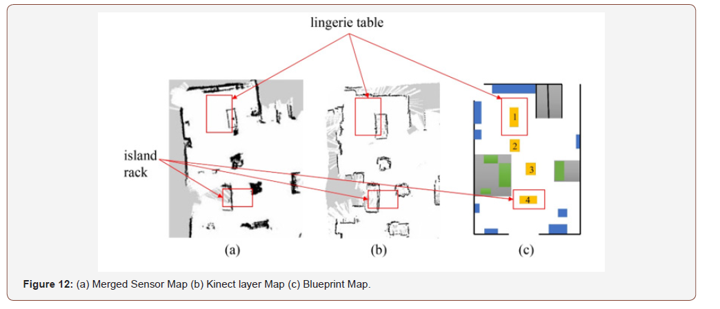
Although the merged-sensor map contains roughly all of the information in the environment, several problems remain. First, walls in the merged-sensor map are distorted, especially the left and right walls. Additionally, the layout in the merged-sensor map is heavily distorted and looks darker (i.e., the lingerie table and island rack). That distortion is caused by inaccurate estimation of self-location. When SLAM updates a map, it first locates itself the robot. When observation data are merged, useful information is lost and SLAM would, thereby, give an inaccurate pose. Based on this inaccurate pose, the updated map is slightly titled. As shown with the lingerie table, inaccurate estimation of the robot pose caused incorrect mapping of the table layout. Consequently, many slightly wrong estimates together make the lingerie table, island rack, and walls look darker. Second, the shapes of obstacles (i.e., the lingerie table) can only be determined if Kinect detects the table repeatedly and the corresponding grid cell in the map can be marked as “occupied”. However, it is hard for the robot to face the table from all directions simultaneously, and as a result, the lingerie table and island rack can only be seen in part.

Compared to the merged-sensor map, our multilayer map is more consistent (or well-registered) with the blueprint map. The walls (boundaries of the whole room) of the multilayer map are very straight and the profiles of obstacles are much more accurate and clearer. The use of LIDAR-estimated pose reduces map distortion, and Kinect provides an abundance of vertical structure information and preserves useful data. The robot updates the observed information combined with a precise pose to get an accurate and complete map. Obviously, the robot performs better using the multilayer algorithm because its location and the structures in environment are precisely estimated.

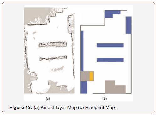
(Figure 13a) shows a Kinect-layer map that was made on another sales floor. Marked in blue in (Figure 13b), there is a table and a rack on the top, and three big shelves on left side and middle of the map. The bottom side has some debris piles (marked in gray. (Figure 13b). These areas are inaccessible to the robot. Most of these obstacles are shown in the Kinect-layer map and the layout of the sales floor is accurate. The multilayer algorithm works well in different environments, and the Kinect-layer map is very accurate when compared with the blueprint map. (Figure 14) (Figure 14a) illustrates a map view of the global path the robot follows during inventory counts, where the green points are the discrete goals of the global path that are generated by the method included in [3]. (Figure 14b) is a photo of the robot navigating a sales floor. The robot is marked by a red rectangle in both (14a) and (14b).

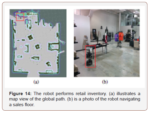
Evaluation of ACO enhanced path planning: Initially, the map generated by our multilayer mapping method was uploaded for the robot to conduct the inventory experiments. We extracted the inventory route covering all RFID tag locations with the global path planner. The robot followed the path to scan all RFID tags within the experimental area (Figure 14). We conducted several experiments to compare the performance of between ACO-enhanced path planning to the RFID inventory path planning method introduced in [3]. Performance is evaluated by two criteria: navigation efficiency and RFID-based inventory accuracy. For all experiments in this section, the ACO was configured with 68 ants and 150 iterations to find the best path.

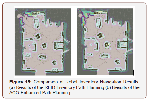
Navigation efficiency: The results of the two paths generated during a typical inventory process are shown in (Figure 15). In this figure, the green points are discrete goals of the global path and the brown curves are the recorded trajectories of the robot that performed an inventory count throughout the store. These trajectories show that the robot moves around products while keeping a safe distance. Additionally, ACO enhanced path planning allows the robot to navigate more efficiently by reducing route overlap. We repeated this experiment five times and compared the average navigational distances and inventory duration by the two (Table 3). For these experiments, the maximum speed of each robot for these experiments was set at 0.7 m/s. As shown in (Table 3), the average inventory duration and navigational distance were significantly reduced with optimization of ACO-enhanced path planning. Inventory count time was optimized by 30.7% and navigational distance was optimized by 28.2%. The difference between the two was caused by varied navigation speeds of the robot as decided by the local planner (or DWA) in the inventory process.

Table 3: Comparison of Inventory Efficiency.

Inventory accuracy: While ACO improves the efficiency of navigation, we tested inventory accuracy using the two path planning methods. We repeated the inventory experiments five times and compared the average accuracy of the two approaches, as shown in (Table 4). Overall, average accuracy with ACO-enhanced path planning was 90.49%. With RFID inventory path planner, average accuracy was 91.53%. To compare, the best accuracy manual inventorying can achieve is in the range of 85 - 90%. Our results show that the ACO-enhanced path planning improves inventory efficiency and that automated inventory accuracy is comparable to manual inventory accuracy.

Table 4: Comparison of Inventory Accuracy.

This paper presents a novel implementation of an autonomous robot for inventory in retail. A multilayer mapping method was introduced as the first step of inventory collection; it fuses sensor observations from LIDAR and Kinect. Rich environmental data provided by Kinect and pose estimation data provided by LIDAR are combined to construct a multilayer map. This provides a robust method for reconstructing and encapsulating complex retail environments that are full of products and shelves of various shapes and heights. Our multilayer mapping method improves the ability of robots to autonomously navigate in complicated environments. Additionally, ACO-enhanced path planning and precision can greatly improve the efficiency of robots that execute RFID-based inventory counts. Lastly, our method maintains count accuracy at the same rate as that of the best manual inventory counts. Thus, our systematic approach is a promising and more cost- and timeefficient implementation of robotic inventory counting.

This work is supported in part by the US NSF under Grant Grant ECCS-1923163, and through the RFID Lab and the Wireless Engineering Research and Education Center (WEREC) at Auburn University, USA.

No conflict of interest.

1. B Hardgrave try it-you’ll like it! the RFID lab’s annual state of adoption report of us retailers, RFID Journal.
2. M Beul, D Droeschel, M Nieuwenhuisen, J Quenzel, S Houben, et al. (2018) Fast autonomous flight in warehouses for inventory applications, IEEE Robotics and Automation Letters 3(4): 3121-3128.
3. J Zhang, Y Lyu, T Roppel, J Patton, C Senthil kumar (2016) Mobile robot for retail inventory using RFID. In: 2016 IEEE International Conference on Industrial Technology (ICIT), IEEE, pp: 101-106.
4. SM Bae, KH Han, CN Cha, HY Lee (2016) Development of inventory checking system based on uav and rfid in open storage yard. In: 2016 International Conference on Information Science and Security (ICISS), IEEE, p: 1-2.
5. WE Davidson (2015) Rail-mounted robotic inventory system. us Patent 9: 129-251.
6. MG Dissanayake, P Newman, S Clark, HF Durrant Whyte, MC sorba (2001) A solution to the simultaneous localization and map building (slam) problem. IEEE Transactions on robotics and automation 17(3): 229-241.
7. T Roppel, Y Lyu, J Zhang, X Xia (2017) Corrosion detection using robotic vehicles in challenging environments. In: CORROSION 2017, NACE International, Louisiana, USA.
8. N Kejriwal, S Garg, S Kumar (2015) Product counting using images with application to robot-based retail stock assessment, In: 2015 IEEE International Conference on Technologies for Practical Robot Applications (Te PRA), IEEE, p: 1-6.
9. TG Zimmerman (2010) System and method for performing inventory using a mobile inventory robot. US Patent 7: 693-757.
10. X Liu, MD Corner, P Shenoy (2011) Ferret: An RFID enabled pervasive multimedia application, Ad Hoc Networks 9 (4): 565-575.
11. J Zhang, Y Lyu, J Patton, SC Peria swamy, T Roppel (2018) Bfvp: A probabilistic uhf rfid tag localization algorithm using bayesian filter and a variable power RFID model, IEEE Transactions on Industrial Electronics 65(10): 8250-8259.
12. MA Bonuccelli, F Martelli (2018) A very fast tags polling protocol for single and multiple readers RFID systems, and its applications. Ad Hoc Networks 71: 14-30.
13. T Brodeur, A Cater, JC Vaz, P Oh (2018) Directory navigation with robotic assistance. In: 2018 IEEE 8^th Annual Computing and Communication Workshop and Conference (CCWC), IEEE, pp: 777-778.
14. G Agnihotram, N Vepakomma, S Trivedi, S Laha, N Isaacs, et al. (2017) Combination of advanced robotics and computer vision for shelf analytics in a retail store. In: 2017 International Conference on Information Technology (ICIT), IEEE, pp: 119-124.
15. J Melià-Seguí, R Pous, A Carreras, M Morenza Cinos, R Parada, et al. (2013) Enhancing the shopping experience through rfid in an actual retail store. In: Proceedings of the 2013 ACM conference on Pervasive and ubiquitous computing adjunct publication, ACM, pp: 1029-1036.
16. B Massimo, R Antonio, R Giovanni, V Andrea (2017) Testing an RFID receiving gate for improving process accuracy in fashion and apparel retail. In: 2017 IEEE 3rd International Forum on Research and Technologies for Society and Industry (RTSI), IEEE, p: 1-5.
17. A Motroni, P Nepa, P Tripicchio, M Unetti (2018) A multi antenna sarbased method for uhf rfid tag localization via UGV. In: 2018 IEEE International Conference on RFID Technology & Application (RFIDTA), IEEE, p: 1-6.
18. I Ehrenberg, C Floerkemeier, S Sarma (2007) Inventory management with an RFID equipped mobile robot. Isn: 2007 IEEE International Conference on Automation Science and Engineering, IEEE, pp: 1020-1026.
19. T Schairer, C Weiss, P Vorst, J Sommer, C Hoene, et al. (2008) Integrated scenario for machine-aided inventory using ambient sensors. In: 4^th European Workshop on RFID Systems and Technologies, VDE, p: 1-8.
20. TH Miller, DA Stolon, JR Spletzer, (2010) An automated asset locating system (aals) with applications to inventory management. In: Field and Service Robotics pp: 163-172.
21. H Durrant Whyte, T Bailey (2006) Simultaneous localization and mapping: part I. IEEE robotics & automation magazine 13(2): 99-110.
22. M Montemerlo, S Thrun, D Koller, B Wegbreit, et al. Fast slam: A factored solution to the simultaneous localization and mapping problem.
23. T Bailey, J Nieto, J Guivant, M Stevens, E Nebot (2006) Consistency of the EKF-SLAM algorithm. In: 2006 IEEE/RSJ International Conference on Intelligent Robots and Systems, IEEE, pp: 3562-3568.
24. Y Lin, J Hyyppa, A Jaakkola (2011) Mini-uav-borne lidar for fine-scale mapping. IEEE Geoscience and Remote Sensing Letters 8(3): 426-430.
25. S Kohlbrecher, O Von Stryk, J Meyer, U Klingauf, (2011) A flexible and scalable slam system with full 3d motion estimation. In: 2011 IEEE International Symposium on Safety, Security, and Rescue Robotics, IEEE, pp: 155-160.
26. LA James, DG Watson, WF Hansen (2007) Using lidar data to map gullies and headwater streams under forest canopy: South carolina, USA, Catena 71(1): 132-144.
27. LM Paz, P Piniés, JD Tardós, J Neira (2008) Large-scale6-dofslamwith stereo-in-hand. IEEE transactions on robotics 24 (5): 946-957.
28. RA Newcombe, S Izadi, O Hilliges, D Molyneaux, D Kim, et al. (2011) Kinect fusion: Real-time dense surface mapping and tracking. In: 2011 IEEE International Symposium on Mixed and Augmented Reality, IEEE, pp: 127-136.
29. J Engel, T Schöps, D Cremers (2014) Lsd Slam: Large Scale direct monocular slam. In: European conference on computer vision, Springer pp: 834-849.
30. M Labbé, F Michaud (2019) RTAB map as an open source lidar and visual simultaneous localization and mapping library for large-scale and long-term online operation. Journal of Field Robotics 36(2): 416-446.
31. R Mur Artal, JMM Montiel, JD Tardos (2015) Orb-slam: a versatile and accurate monocular slam system. IEEE transactions on robotics 31(5): 1147-1163.
32. J Zhang, S Singh (2015) Visual lidar odometry and mapping: Low-drift, robust, and fast. In: 2015 IEEE International Conference on Robotics and Automation (ICRA), IEEE, pp: 2174-2181.
33. EY Lee, HJ Cho, KY Ryu (2016) A probabilistic approach for collision avoidance of uncertain moving objects within black zones. Ad Hoc Networks 52: 50-62.
34. L Liu, G Han, H Wang, J Wan (2017) Obstacle-avoidance minimal exposure path for heterogeneous wireless sensor networks. Ad Hoc Networks 55: 50-61.
35. R Dai, S Fotedar, M Radmanesh, M Kumar (2018) Quality aware uav coverage and path planning in geometrically complex environments. Ad Hoc Networks 73: 95-105.
36. PE Hart, NJ Nilsson, B Raphael (1968) A formal basis for the heuristic determination of minimum cost paths. IEEE transactions on Systems Science and Cybernetics 4(2): 100-107.
37. LE Kavraki, P Svestka, J Latombe, MH Overmars (1996) Probabilistic roadmaps for path planning in high-dimensional configuration spaces.
38. LE Kavraki, J claude Latombe (1998) Probabilistic roadmaps for robot path planning.
39. SM Lavalle (1998) rapidly exploring random trees: A new tool for path planning, Tech rep, USA.
40. K Yang, S Keat Gan, S Sukkarieh (2013) A gaussian process based rrt planner for the exploration of an unknown and cluttered environment with a UAV, Advanced Robotics 27(6): 431-443.
41. M Mitchell (1998) An introduction to genetic algorithms, MIT press, USA.
42. S Kirkpatrick, CD Gelatt, MP Vecchi (1983) Optimization by simulated annealing. science 220(4598): 671-680.
43. M Dorigo, M Birattari (2010) Ant colony optimization algorithms.
44. HH Mukhairez, AY Maghari Performance comparison of simulated annealing, GA and ACO applied to TSP. Performance Comparison of Simulated Annealing, GA and ACO Applied to TSP 6(4).
45. SA Haroun, B Jamal (2008) A performance comparison of ga and aco applied to TSP. International Journal of Computer Applications 117(20).
46. A Doucet, N De Freitas, K Murphy, S Russell (2000) Rao black wellised particle filtering for dynamic bayesian networks. In: Proceedings of the Sixteenth conference on Uncertainty in artificial intelligence, Morgan Kaufmann Publishers Inc pp: 176-183.
47. S Thrun, D Fox, W Burgard, F Dellaert (2001) Robust monte carlo localization for mobile robots. Artificial intelligence 128(1-2): 99-141.
48. Slamtec, Rplidar (2018) A1 Low Cost 360 Degree Laser Range Scanner Introduction and Datasheet, rev 1.1(3).
49. K Kamarudin, SM Mamduh, AYM Shakaff, SM Saad, A Zakaria, et al. (2013) Method to convert kinect’s 3D depth data to a 2D map for indoor slam. In: 2013 IEEE 9^th International Colloquium on Signal Processing and its Applications, IEEE, pp: 247-251.
50. MF Fallon, H Johannsson, J Brookshire, S Teller, JJ Leonard (2012) Sensor fusion for flexible human-portable building-scale mapping. In: 2012 IEEE/RSJ International Conference on Intelligent Robots and Systems, IEEE, pp: 4405-4412.
51. M Zaratti, Rfid sensor (2007).
52. DM Dobkin (2012) The rf in RFID: uhf RFID in practice, Newness, USA.
53. D Fox, W Burgard, S Thrun (1997) The dynamic window approach to collision avoidance, IEEE Robotics and Automation Magazine 4(1): 23-33.
54. L Wong, NH Moin (2015) Enhanced ant colony optimization for inventory routing problem. AIP Conference Proceedings 1682(1): 030007.
55. G Ye, X Rui (2013) An improved simulated annealing and genetic algorithm for tsp, In: 2013 5^th IEEE International Conference on Broadband Network & Multimedia Technology, IEEE, p: 6-9.
56. M Dorigo, LM Gambardella, M Middendorf, T Stutzle, (2002) Guest editorial: special section on ant colony optimization, IEEE Transactions on Evolutionary Computation 6(4): 317-319.
57. R Bajaj, V Malik (2000) A review on optimization with ant colony algorithm, Journal of Network Communications and Emerging Technologies (JNCET).
58. M Dorigo, L M Gambardella (1997) Ant colony system: a cooperative learning approach to the traveling salesman problem, IEEE Transactions on evolutionary computation 1(1): 53-66.
59. FJ Vasko, J Bobeck, M Governale, D Rieksts, J Keffer (2011) A statistical analysis of parameter values for the rank-based ant colony optimization algorithm for the traveling salesperson problem, Journal of the operational Research Society 62(6): 1169-1176.