


 Review Article
Wealth Inequality in the US - The Role of Housing
Received Date: April 02, 2024; Published Date: April 12, 2024
Abstract
What is the role of wealth inequality in causing and amplifying business cycles & vice-versa? Can we quantify the correlation between housing and estimated business cycle shocks & frictions along the lines of Bayer, et al. [1,2] with its subsequent impact on business-cycles & the time-varying wealth distribution? I propose to estimate a heterogeneous-agent New-Keynesian (HANK) model in continuous time featuring two illiquid assets and gross positions for housing. The model emphasizes the differential impacts of asset price changes suitably calibrated to match key features of the observed US wealth distribution. The constructed counterfactuals are intended to have strong implications for the redistributive role of monetary & fiscal policy in impacting the wealth-shares of both the top 10% & middle 50-90% in the post-pandemic era.
Keywords: Inequality; heterogeneous agents; mortgage; Housing Supply and Markets
JEL Codes: D63; E31; G28; G51; R38; R31
Introduction
The new class of HANK models imply new transmission channels of monetary as well as fiscal policies operating primarily through household portfolio decisions. The additional principal advantage of HANK models is their ability to study the timevarying joint distributions of wealth & income. Recently, literature has made significant breakthroughs in applying the business cycles shocks & frictions estimated in the seminal work of Smets and Wouters [3] analogously to HANK models. Bayer, et al. [1,2] comments on the relation between wealth inequality & business cycles by focusing exclusively on the top 10% income & wealth shares1. They use annual data from the World-Inequality database (WID) for the period 1954-2019 for the corresponding measure of inequalities with little structural focus on housing. Subsequently, the data is combined with oft used quarterly macroeconomic time series for the Bayesian likelihood estimation of various HANK models. Surprisingly, they find that additional cross-sectional information on inequality has mattered little for business cycles. I propose an alternative modeling setup with richer depiction of household portfolio heterogeneity to match both the 50-90% & top 10% of the wealth distribution. The goal of the exercise would be to consequently comment on the interlinkage between housing, wealth inequality & business cycle drivers2.
There is ample empirical evidence for the heterogeneity in household portfolios and its consequent importance for the evolution of the US wealth distribution over time. Kuhn, et al. [4] document how the heterogeneous impact in asset price shifts have led to the secular increase in wealth inequality post GFC which has contributed to the decoupling between the income & wealth distributions. They report that the bottom 90% have portfolios dominated by housing while the top 10% own predominantly corporate & non-corporate equity3. The bottom 50% of the wealth distribution have little net wealth. Yet, their net nominal position masks substantial gross positions which is highly levered. The highly levered position in housing is another common feature they share with their counterparts in the 50-90% quantiles of the distribution who have increasingly positive net wealth. This is in contrast with the top 10%, the subject of study in Bayer, et al. [1,2]. The latter report asset price movements are driven by estimated idiosyncratic productivity shocks.
This would be consistent in the absence of additional elements of household portfolio heterogeneity. They are silent on the impact on the bottom 90% for whom the house is the single most important asset. The evidence motivates me to focus on both the 50-90% & the top 10%. Literature has recently made tremendous progress in successfully matching both parts of the time-varying wealth distribution simultaneously in the absence of business cycle shocks & frictions. On the structural side, recently Humber, et al. [5] have articulated the importance of declining tax progressivity in shaping the US wealth distribution using a heterogeneous agent macroeconomic model. The observed variation in asset returns propagating through the heterogeneity in household portfolios is the key to matching simultaneously both the middle & top parts of the observed wealth distribution. Their model features two discount factors and a single asset. The dynamics also prove to be successful in replicating the empirical patterns. However, they abstract from incorporating business cycle shocks & frictions & their consequent interdependence, quite extensively investigated in Bayer, et al. [1,2]. Since discount factor heterogeneity is hard to measure, my model alternately relies on approaching the problem using 2 illiquid assets on the household side suitably calibrated to match key moments of the wealth distribution. Wealth distribution is a slow-moving variable where small shocks accumulate over time and provides the motivation for exploiting the differences between a house and corporate & non-corporate equity, particularly the rate at which the respective asset owners realize their returns. Subsequently, this would lead to divergent trends in the rates of motion of the different quantiles of the wealth distribution. The setup is both intuitive and capable of modeling the interactions with the observed macroeconomic data. It also allows for a more comprehensive review of policy options to which I turn to next.
Foot Notes
1 Another important paper in this context who have built on the alternate approach of Boppart et al. (2018) is Auclert et al. (2019).
2 I abstract from commenting on the same about income inequality. Auclert and Rognlie (2018) & the literature that follows look exclusively at the correlation between income inequality & aggregate demand.
3 Similar complimentary evidence is documented by Kuhn et al. (2016) & in their updated results till 2020 (most specifically, Table 5).
The stark implications for both monetary and fiscal policy in incomplete market frameworks have been documented in the seminal contribution of Kaplan, et al. [6] who use a state of the art twoasset HANK. calibrated to match the observed net wealth positions across the entire distribution. They, and the majority of literature that followed, have abstracted from the computational difficulties in modeling a richer household portfolio with the perception of realizing very little gains. However, as I intend to demonstrate with this proposal, a two-asset framework with the illiquid asset earning the same rate of return is incompatible with reality. They matter more for my present purposes where the heterogeneity in both the observed holdings of the two illiquid assets & their returns are majorly responsible for the divergent trends in the different parts of the US wealth distribution. In particular, a house is often the only source of insurance for the 50-90% of the distribution unlike the top 10%. Transactions in housing are infrequent motivating larger adjustment costs and it is significantly less liquid as compared to other illiquid assets that dominate portfolios of the top 10%. It also brings the role played by the wealthy hand-to-mouth who dominate the 50-90% to the forefront allowing for richer dynamics in the wealth distribution, both for the steady state & along the transition path. My preliminary modeling environment aims to isolate the role of housing in contributing to the wealth dynamics through gross positions in illiquid assets. The empirical motivation behind the choice of gross over net returns for asset positions has been aptly justified by Bach, et al. [7] who show that the expected return on gross wealth strongly increases with net worth, primarily because wealthy households bear high systematic risk. By contrast, the expected return on net wealth is flat across most of the distribution because the middle class holds levered positions in real estate. This carries over to the shares of systemic & idiosyncratic risks borne by different parts of the distribution. The expected return on net wealth turns significantly lower in the middle of the distribution which motivates the choice for using gross housing positions. The framework would unfortunately display an increase in the dimensions of the state space which I hope to reduce following the techniques developed by Ahn, et al. [8]4. Using a mixture of calibration & estimation, I propose to subsequently see the correlation between rates of return on housing & stock prices with the whole gamut of estimated business cycle shocks with its implications for tracing the wealth distribution. In contrast to the GFC which was triggered by falling house prices leading to a very large negative unemployment shock, the Covid-19 crisis originated in the labor markets as a large transitory increase in unemployment; some of which is expected to be persistent. Fresh stock market booms have coincided with a near-record rise in house prices from a chronic undersupply of houses coupled with mortgage rates falling to historic lows. The unique nature of the joint shock has not only interesting implications for the evolution in wealth inequality going forward but also offers a natural environment for an event study into the behaviour of interest rates & wealth inequality. The housing boom of the 2000s remains one of the few instances where the realized returns for the 50-90% quantiles kept up pace with the corporate equity returns for the top 10%. This slowed the rise in wealth inequality as demonstrated in Kuhn, et al. [4]. The proposed environment should match the GFC wealth distribution to see the implications for the current crisis. In particular, the two parts of the distribution are predicted to be moving at nearly the same rate. The task is helped by the behaviour of monetary policy which can be viewed as purely exogenous to portfolio returns currently. The proposed mixture of calibration & estimation also offers additional normative lessons for policy makers. The rest of the proposal is divided into 4 parts. Section 2 gives a brief description of the modeling environment, mathematical details of which are contained in A. Sections 3 & 4 focus on calibration & estimation respectively. Section 5 concludes with possible applications in investigating the time-varying dynamics of wealth inequality.
Model
The model is setup in continuous time5 which offers several advantages over discrete time. The proposed setup is based on Kaplan, et al. [6]. I list here all the changes with the bulk of the modification introduced in household portfolio heterogeneity in section 2.1. There has been very little work on the Bayesian estimation of continuous time HANK models which I feel is a huge motivation in itself. I am hoping to combine the procedure in both Ahn, et al. [8] & Bayer, et al. [1,2] as the first steps in making the framework feasible. The primary aim is to model time-varying wealth distributions using two distinct illiquid asset classes. Income inequality will be produced solely by the earnings process at steady state. Its consequent interactions with estimated business cycle frictions & added cross-sectional information will determine in part the transition path of the wealth distribution. Equations detailing the steady state & sources of exogenous shocks are listed in Appendix A.
Foot Notes
4 The procedure also allows for the introduction of aggregate shocks. Discrete time techniques for model reduction have been investigated in Bayer and Luetticke (2020) (used by Bayer et al. (2020)) & Auclert et al. (2019).
5 Achdou et al. (2017) gives a comprehensive discussion for adopting & solving (both theoretically & numerically) heterogeneous agent models in continuous time.
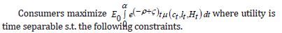
Households
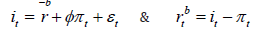
There is a continuum of households indexed by their holdings of liquid assets b, illiquid houses H, other illiquid assets and their idiosyncratic labor productivity z. Time is continuous, and the state of the economy can be characterized by a joint distribution ì t (da, dH, db, dz) . The utility function is modified to induce households to invest in the house before holding other illiquid assets. Households receive utility from consuming and disutility for labor supply. Households can borrow in liquid assets up to an exogenous limit at some real rate of interest that is associated with the return on liquid assets (rtb ) . The borrowing wedge introduced gives additional freedom during calibration to ensure the model can generate empirically plausible mass of individuals at the borrowing limit. The liquid assets are invested in government bonds offering the return rtb . Households maximize utility subject to the laws of motion for the liquid and other illiquid assets while satisfying their borrowing limits.
Housing as a separate class of illiquid assets
All agents prefer to invest in owning a house than investing all their wealth in illiquid assets. The utility from the former is far greater. To simplify, the 50-90% only own a house while the top 10% hold other illiquid assets post sufficient investment in housing. There is no substitutability between the two illiquid asset classes which reduces state space dimensions. Housing can be bought through savings or borrowing of liquid assets (implicitly the mortgage). This makes the effects of exogenous portfolio price changes sharper & enables gauging their impact on the wealth distribution. For modeling purposes, housing is very illiquid and asset price gains can be extracted after paying substantial transaction costs. This key feature separates houses from other illiquid assets which can be transacted much more freely as in practice. I intend to have a discrete time Poisson process for the very slow movements in the housing stock to capture these effects. The earnings process for the households is retained. This endogenously builds in the effects of income-inequality to wealth inequality (more details in section 3.1).
Two different Adjustment Cost Functions
There are now two distinct adjustment cost functions. I envision a similar functional form as in [6]. It is substantially easier to convert t at into bt and vice versa in contrast with housing transactions. The individual pays hefty transaction costs that capture both the search & matching involved as well as the extremely illiqiuid nature of the housing market6. The difficulty in converting house price gains into liquid assets & adding to housing positions underlies the key mechanism behind the time divergent trends in the wealth distribution from portfolio price changes. The distribution for the 50-90% is now an extremely slow moving object unlike the top 10% who can rapidly convert their holdings of equity into liquid assets & vice-versa in response to booming stock markets. The same cannot be said for housing. As remarked earlier in section 1, the housing boom pre-GFC remains the only major exception. The mortgage can also be a source of the changing stock of housing through the refinancing & home equity extraction channels. This is available only for a select set of households who qualify by paying the necessary transaction costs. The parameters in the adjustment cost function can be hopefully calibrated if such impacts are to be of first order importance in the future. The presence of 2 separate adjustment cost functions is the major transmission mechanism that essentially drives the dynamics of wealth inequality over time. The setup is designed to capture the distinct role of housing and will be majorly responsible for the transition paths to policy experiments and estimated shocks as detailed in section 5.
Rest of the Economy
I retain the production structure as in Kaplan, et al. [6]. This creates some dissimilarities with Bayer, et al. [1,2] where there are four differentsubgroupss of firms. The retained earnings channel is majorly responsible for their success in matching the wealth distribution of the top 10%. It is missing from this setup with the production structure being modelled in a more conventional form. There are only two groups, final & intermediate producers. The labor & wage risks are therefore also likely to be underestimated. Here the question of interest is whether a richer depiction of household portfolio in line with empirical evidence is sufficient for generating plausible wealth distributions in the absence of substantial supply side mechanisms. It remains very much a model focusing on the demand side forces. Secondly, it would be interesting to study the enriched demand side aggregation in the presence of similarly estimated business cycle frictions. The role of the government and monetary authority is the same as in [6].
General Equilibrium modifications
Closing the model requires partly determining how the
illiquid savings will be invested besides the normal market
clearing conditions. The former is majorly different under my
setup due to the presence of two illiquid assets. The setup is also
not designed to test the equity premium puzzle. Alternately, it
takes the asset returns as exogenous and observes its impacts on
the holdings of illiquid assets. I will assume that the house (Ht)
cannot be converted into liquid assets that can be channel led
into investing in physical capital while other illiquid assets (at) can be freely transformed. The return on equity (at) determines
the rate of return on capital 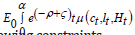 which controls the capital stock
accumulation in the economy. Higher returns on equity motivate
higher holdings of at which leads to increased capital accumulation
& a decrease in its rate of return. Specifically, keeping the notation
as close as possible to Kaplan, et al. [6],
which controls the capital stock
accumulation in the economy. Higher returns on equity motivate
higher holdings of at which leads to increased capital accumulation
& a decrease in its rate of return. Specifically, keeping the notation
as close as possible to Kaplan, et al. [6], 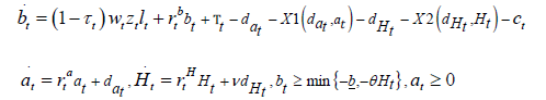 The 50-90% of
the distribution plays no role. Implicitly, stock market booms lead
to higher higher capital accumulation which increases the wage.
Labor supply also increases, and overall output goes up. The
setup is closer to the traditional model of Aiyagari [9]. Though its
admittedly stylized, post GFC when the the vast majority had to
delever, the top 10% have been indirectly funding the rest of the
distribution [10]. The overall calibration therefore should not be
very different, and I hope to avoid any counterfactual volatilities in
consumption, investment and output.
The 50-90% of
the distribution plays no role. Implicitly, stock market booms lead
to higher higher capital accumulation which increases the wage.
Labor supply also increases, and overall output goes up. The
setup is closer to the traditional model of Aiyagari [9]. Though its
admittedly stylized, post GFC when the the vast majority had to
delever, the top 10% have been indirectly funding the rest of the
distribution [10]. The overall calibration therefore should not be
very different, and I hope to avoid any counterfactual volatilities in
consumption, investment and output.
Foot Notes
6 One of the few papers that looks solely at issues of the housing market in a HANK setup is Hedlund et al. (2017) who focus on the interaction of housing debt with liquidity traps.
State Space Reduction & Aggregate Shocks
An equilibrium here is the tuple 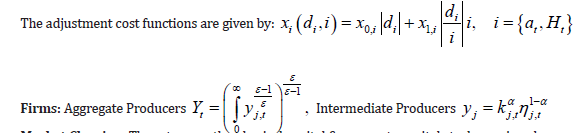 subject to the input prices
,exogenously specified returns
subject to the input prices
,exogenously specified returns 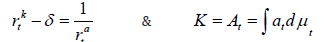 inflation
 measures capturing the distribution
 fiscal
 and aggregate quantities such that
following Kaplan et al. (2018), at every t : (a) households and firms
maximize their objective functions taking as given equilibrium
prices, taxes, and transfers; (b) the sequence of distributions
satisfies aggregate consistency conditions; (c) the government
budget constraint holds; and (d) all markets clear. There are no
aggregate shocks at the steady state. Since there are two illiquid
assets, I hope to reduce the state space following the methods of
Ahn, et al. [8]. Not all the parameters are required for computing
the stationary distribution. The required parameters are calibrated
according to section 3. The equilibrium conditions are linearized
and the state space is made computationally feasible for dynamics.
The aggregate shocks & parameters which solely affect dynamics
can now be estimated (section 4). Additional aggregate shocks can
be also introduced to bring the model closer to Bayer, et al. [1,2].
and aggregate quantities such that
following Kaplan et al. (2018), at every t : (a) households and firms
maximize their objective functions taking as given equilibrium
prices, taxes, and transfers; (b) the sequence of distributions
satisfies aggregate consistency conditions; (c) the government
budget constraint holds; and (d) all markets clear. There are no
aggregate shocks at the steady state. Since there are two illiquid
assets, I hope to reduce the state space following the methods of
Ahn, et al. [8]. Not all the parameters are required for computing
the stationary distribution. The required parameters are calibrated
according to section 3. The equilibrium conditions are linearized
and the state space is made computationally feasible for dynamics.
The aggregate shocks & parameters which solely affect dynamics
can now be estimated (section 4). Additional aggregate shocks can
be also introduced to bring the model closer to Bayer, et al. [1,2].
Calibration
The goal of the model is to have a properly calibrated wealth distribution that would match the key moments (more details in section 3.3) for both the middle 50-90% & the top 10% of the US wealth distribution. It should be for a suitable time period that would allow for a clean comparison with both the existing HANK models of Kaplan, et al. [6] & Bayer, et al. [1,2]. Firstly, it would allow me to see the impact on parameter estimates of shocks that commonly drive business cycles with additional robust inequality data. This answers the first question of whether business cycles matter for wealth inequality. Secondly, it allows me to study the accuracy from incorporating additional cross-section information on simultaneously matching both the stock of housing & other illiqiuid assets that proxy for the two parts of the wealth distribution simultaneously (section 4). Both the results would enrich the literature along the dimensions of Bayer, et al. [1,2]. Matching observed income inequality is not the focus and it is likely that the model will produce counterfactual income distributions in an attempt to focus solely on the wealth distribution. The proposed framework departs majorly from the 2-asset HANK of Kaplan, et al. [6] by assuming 5 gross asset positions instead of net7. The production side is more or less standard and I would follow their calibration. Same goes for the most of the remaining model parameters relating to demographics, preferences, government and monetary policy (details of which are presented in section D of their paper). The parameters that have not been calibrated can be estimated using the likelihood estimation procedure in section 4.
Earnings dynamics
The continuous time earnings process is cutting edge in Kaplan, et al. [6] and I would prefer to retain it8. The skewed earnings distribution is responsible for generating the skewness in the distributions of both the liquid & illiquid assets. The earnings process is likely to remain the same for my setup and have minimal deviations. A big advantage of using this earnings process is to eliminate additional cross-sectional information on income risk. I suspect not having a similar process in Bayer, et al. [1,2] is majorly responsible for their singular result that inequality data do not not affect business cycles. Here, the income risk is prebuilt and the framework allows for its potential rich interactions with the estimated business cycle frictions. It simplifies the causal impact of income inequality on wealth distributions, the focus of the proposal.
Categorization of Assets into Liquid and Illiquid
I would retain their mapping of classifying assets for the household sector into liquid vs illiquid with the major change of focusing on gross positions instead of net positions. This changes the definition of housing which had two different components: the real estate wealth and the mortgage debt. To keep the focus on first order effects, I would calibrate the illiquid asset positions on housing to the real estate wealth. The borrowing in liquid assets can be calibrated for the mortgage position. This would capture the direct impact of asset price effects on the stock of housing. Recognized both empirically & theoretically to be a powerful driver of wealth inequality, it is potentially massively underestimated using net positions. Since almost 98% of US mortgages are FRM9, any endogenous/exogenous change in mortgage rates & house prices is likely to have only second-order impacts on the borrowing in liquid assets. Alternate calibration of considering gross liquid & other illiquid assets is unlikely to change any result significantly for the 50-90% who are heavily dependent on housing. Similarly, gross over net position on corporate & non-corporate equity is also unlikely to cause any major difference since the top 10% of the distribution have very little debt. To keep it simple, I would calibrate the rest of the assets to net positions as followed by Kaplan, et al. [6].
Foot Notes
7 The gross position of housing enables sizeable redistribution through monetary policy channels through the concept of unhedged interest rate exposures, Auclert (2019).
8 They estimate the earnings process by Simulated Method of Moments using Social Security Administration (SSA) data on male earnings from Guvenen et al. (2015).
9 Source: Origination Report Ellie Mae (2021) https://static.elliemae.com/pdf/origination-insight reports/ICE_OIR_ JAN2021.pdf.
The adjustment cost functions
The adjustment cost function has been calibrated to match the five moments of the distribution of household wealth: the mean of the illiquid and liquid wealth distributions, the fraction of poor and wealthy hand-tomouth [11] and the fraction of households with negative net liquid assets (which identifies the borrowing wedge). Here, there would be two different adjustment cost functions controlling the decisions for the two parts of the wealth distribution. There are additional degrees of freedom where we can allow for the different rates of return to the two illiquid assets to play out its implications for the model (section2.1.2) or control it by suitably altering. I prefer to start with the case of having two different forms but a counterfactual could be constructed to get a true measure of the impact of the differential rates of return on the heterogeneity in household portfolios in the steady state as well as the true importance of adding the second illiquid asset (which is housing).
Estimation
Bayer, et al. [1,2] use quarterly US data from 1954Q3 to 2019Q4 and include the following eight observable time series in the baseline: the growth rates of per capita GDP, private consumption, investment & wages, all in real terms; the logarithm of the level of per capita hours worked; the log difference of the GDP deflator and the (shadow) federal funds rate. All the variables are demeaned so the model is stationary. Annual data on the top 10% income & wealth shares are obtained from the World Inequality Database (WID). Other data at shorter time frames on income risk and tax progressivity which have been directly estimated are included. However, since the model already possesses a cutting-edge earnings process, I plan to exclude the income risk data from the set of cross-sectional information. Alternatively, I propose to include firstly the data of the 50-90% wealth & income shares from the WID along with the measures on tax progressivity. Since the estimating framework allows for mixed-frequency, relevant data from Kuhn, et al. [4] to allow for richer representations of the portfolio price channels would be value-added. Particularly, a subset of the data for the heterogeneity of the household portfolios corresponding to Figures 12B, 13, 14B & C, 15−19 in their paper would allow me to study the correlation with the set of estimated shocks as well as give some indications about the causality. Most of the parameters for the standard business cycle shocks and frictions are estimated. The prior distributions are taken from previous literature. I hope to follow a similar approach for the parameters which were not calibrated in my framework. The model with the augmented data can be hopefully estimated by a full information Bayesian likelihood approach using the state-space representation of the model which allows for mixed-frequency data using an identical methodology. In particular, the paper uses a Kalman filter to obtain the likelihood from the state-space representation of the model solution and employ a standard random walk Metropolis-Hastings (RWMH) algorithm to generate draws from the posterior likelihood10. They also provide convergence statistics as well as traceplots for the individual parameters of the various models estimated.
Planned Exercises
Since the procedure for estimation that I propose to adopt is identical to Bayer et al. [1,2], the analysis along the transition path will be of a similar nature that is detailed in section 4 of their paper. The variance decomposition exercises have been performed for a particular year as well as historically. Besides matching the income & wealth distributions, the exercises were carried out for all observables like output, consumption, investment, etc. I list here the differences that arise due to the tweaks in the modeling setup and focus specifically on the observable wealth shares of the top 10% & middle 50-90%.
Without any cross-sectional data
First and foremost, I plan to check the impact on wealth inequality from estimating the model without any cross-sectional data and illustrate the findings using a series of variance decomposition plots. I hope to achieve three sets of results. Firstly, the inclusion of a richer depiction of household portfolio heterogeneity with a well calibrated earnings dynamics has a good chance of improving the importance of business cycle shocks for wealth inequality for the top 10% in an improvement over Bayer, et al. [1,2]. Secondly, the estimated frictions, for the same reasons, will now be insufficient to explain variables like output, investment & consumption. Thirdly, I intend to demonstrate that estimated business cycle frictions are insufficient to model both the 50-90% & top 10% of the wealth distribution simultaneously. Different parts of the wealth distribution contain idiosyncratic structural trends that are unlikely to be majorly caused by the seven” standard” shocks along the lines of Smets and Wouters [3]11. Empirical analysis indicates that these trends are heavily correlated with differential movements in asset prices. With the exception to maybe monetary policy shock in recent times, they are (especially house prices) are unlikely to be dependent on the set of business cycle shocks. It may be concerning that the risk premium shock may be capturing the differential asset price movements, but I believe it would be insufficient in the absence of explicit cross-sectional data on the same. It would instead capture the precautionary savings motive. This is unlikely to have any major implications for the wealth distribution which moves along sluggishly accumulating shocks. The set of seven shocks would perhaps be enough to model income inequality without the need for additional cross-sectional data but that is outside the purview of the current proposal.
Foot Notes
10 More details about their procedure is contained in An and Schorfheide (2007) & Fern´andez-Villaverde (2010).
11 Specifically, the seven shocks are TFP, investment specific technology, price markup, wage markup, risk premium, monetary policy & structural deficit (government budget deficit).
Effect of additional cross section information
Before adding cross-sectional information, the unspecified risk premium is likely to remain the single largest component in the variance decomposition. Adding cross-sectional information one at a time helps in isolating the marginal impact of each factor. Data on wealth & income shares of 50-90% along with existing top 10% is expected to give the least improvements. The main focus is the data on asset prices & the exposure of the two parts of the distribution to house prices. Similar arguments can be made for the data on tax progressivity (major reason as per Hubmer, et al. [5]) which may be included if the previous results are promising. Another interesting exercise would be to see the joint impact of tax progressivity & asset price differentials in conjunction with the set of business cycle frictions (all together or 2 at a time). This can be repeated similarly for the historical decomposition of the wealth distribution. Crosssectional information can be also used to determine the causality between inequality & estimated business cycle frictions. I hope at least the portfolio price changes will be a major causal indicator for the monetary policy & risk premium. This would generate intuitive results and emphasize the need for additional complexity in modeling the household portfolio heterogeneity.
Historical decompositions of US wealth inequality
Larger income risks and sharply increasing markups after the 2000s led to the firms having higher retained earnings, a factor modeled to improve the accuracy in matching US wealth inequality. A part of income inequality also translates to wealth inequality which occurred through the addition of cross-sectional income risk, a feature absents in my proposed model. Instead, as referenced before in section 2, I am relying onthe income dynamics pre-built to measure the pass-through of income inequality to wealth inequality. This also has the advantage of being a more realistic framework to gauge the true impact of business cycle frictions on the timevarying wealth distribution in the absence of any cross-sectional data. The explicit asset pricing channel that I propose to introduce would become majorly important for the GFC. In the terms of Bayer et al. [1,2], this has been modeled as an estimated technology shock to mimic the top 10% wealth inequality. However, they concur on the importance of the independent role played by change in asset prices. As mentioned towards the end of section 1, the performance of my proposed modeling framework can be judged therefore on the ability to match both parts of the distribution simultaneously around the GFC. A good performance would enable the environment to be taken considered for normative policy prescriptions.
Counterfactuals on wealth inequality
Another major motivation behind the study of the current proposal is the interlinkage between asset price changes & the behaviour of interest rates post GFC. I plan a counterfactual of the importance of a prolonged horizon of very low interest rates (a very large positive & persistent estimated monetary policy shock) to the evolution of the wealth distribution for both the middle 50-90% & top 10% and also its dependence with changing asset prices that has been introduced as additional cross-section information. The model will be calibrated to match the GFC era wealth distribution before the start of the experiment. The second counterfactual of similar nature would involve using rapidly rising public debt (again a very large positive & persistent shock to estimated structural deficit). An interesting feature to note in this context would be the behaviour of the risk premium and whether the impulse responses would be consistent with the evidence on the savings glut of the rich as put forth in Mian, et al. [10-21] by studying the impact on particularly the top 10% wealth share. Third, the natural extension would be the joint shock which approximately describes the exogenous behaviour of monetary & fiscal policy for the postpandemic era. The rare event study allows for clean identification for the source of shock on the wealth distribution. It acts primarily through asset prices & risk premium channel for first order effects and has the potential to be one of the cornerstone normative results of this proposal, if successful.
Conclusion
In this planned study, the role of wealth inequality in influencing and being affected by business cycles is explored through a sophisticated model that incorporates heterogeneity in household portfolios and simulates the effects of various economic shocks and policy measures on wealth distribution. The analysis, grounded in a novel Heterogeneous Agent New Keynesian model with three different assets, reveals nuanced insights into how business cycle shocks, particularly those related to housing and asset prices, differentially impact the wealth distribution among the top 10% and the middle 50-90% brackets. The planned exercises and counterfactual scenarios, informed by past research and adapted to consider specific nuances of wealth inequality, aim to quantify these effects with a high degree of precision. Through historical decompositions and the consideration of additional cross-sectional data, this research sheds light on the complex interplay between monetary and fiscal policies and wealth inequality, especially in the context of post-pandemic economic recovery. The findings would underscore the importance of asset price changes and policy interventions in redistributing wealth, suggesting that targeted policy measures could mitigate the adverse effects of business cycles on wealth inequality.
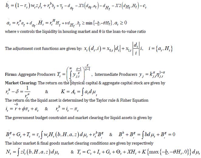
A Model Equations for Equilibrium
Households: Households in the 50-90% of the distribution cannot afford other illiquid assets. This can be controlled by some threshold value of idiosyncratic income risk to ensure bt = 0 for any household occupying the middle quantiles.
Besides the seven estimated shocks based on the US time series data, additional parameters which have not been calibrated but affect the dynamics can be divided into four lists according to Bayer, et al. [1,2]: Frictions, Debt & monetary policy rule shocks, Tax rules (for measuring tax progressivity) and other structural shocks (sections 3.3 and 3.4 of their paper has more details). The prior distributions are obtained following the literature. The setup here has to be suitably amended to include the necessary parameters that need to be assessed. The list of income risks is missing since the earnings process already incorporates it in this modeling framework.
Acknowledgements
I would like to extend my gratitude to my primary advisors Professors Yu-Chin Chen and Brian Greaney for their invaluable time, advice, and assistance with this project. I am also thankful to my committee members, Professors Fabio Ghironi and Stephen Turnovsky, for their insightful suggestions.
Conflict of Interest
No financial or any conflict of interest.
References
-

This work is licensed under a Creative Commons Attribution-NonCommercial 4.0 International License.


