Digital Finance and Structural Transformation: Analyzing the Influence of Emerging Financial Indicators on Retail Sector Expansion in China

The evolution of China’s digital economy has redefined conventional economic models, with financial metrics significantly influencing retail sector growth and national economic outcomes. This study examines the impact of emerging financial performance indicators, including Broad Money (BM), Foreign Direct Investment (FDI), Market Capitalization (MC), and Research & Development Expenditures (RDE) on the growth of Gross Domestic Product (GDP) in the framework of a digitally enabled retail economy. The study used Ordinary Least Squares (OLS), Principal Component Analysis (PCA), and Ridge Regression on data spanning from 2012 to 2021 to quantify both direct and elasticity-based correlations between financial measures and GDP with elasticity-based analysis demonstrating that a 1% increase in R&D resulted in a 0.62% gain in GDP. The model had substantial explanatory power (adjusted R² = 0.803). Significant findings indicate that heightened R&D investment and foreign direct investment are favorably correlated with GDP growth and play a crucial role in fostering innovation-driven retail expansion. The findings demonstrate that market capitalization significantly affects digital consumption patterns and capital influx into retail- focused services. The paper finishes with policy recommendations aimed at fortifying digital finance, augmenting investment avenues, and fostering innovation in retail marketplaces, so establishing China’s retail industry as a pivotal driver of sustainable economic growth.

Keywords:GDP growth; financial key performance; digital economy; china retail sector; economic development

The rise of China as a global leader in digital transformation has profoundly influenced the financial and retail sectors. The integration of digital money into retail activities is central to this transition, redefining consumer interactions with services and products. As retail platforms become more influenced by digital payments, e-commerce, AI-driven personalization, and crossborder digital trade, financial indicators have acquired heightened significance in assessing macroeconomic results. In China, the advancement of a digitally driven economy has cultivated a distinctive correlation between financial innovation and GDP growth, particularly in sectors such as online retail and service delivery. Conventional financial measures like Broad Money (BM), Foreign Direct Investment (FDI), and Market Capitalization (MC) have increasingly impacted consumer markets, influencing demand, innovation, and logistical efficiency. The strategic significance of Research & Development Expenditures (RDE) in promoting digital retail innovation, encompassing Fin-tech solutions and automated fulfillment, underscores the confluence of financial and consumer service trends. China is also diligently promoting the digital economy and making substantial efforts to establish a digital China [1]. The importance of digital finance as a crucial sector of the economy is undeniable. The national economy of China is increasingly dependent on digital finance as a vital driver and source of advancement [2]. The Chinese miracle denotes the 9.4% annual growth rate of China’s gross domestic product (GDP) since its reform and liberalization, which has elevated the nation to the status of the world’s second-largest economy. To ensure equitable access to the benefits of the digital economy, initiatives are underway to bridge the digital divide within the country. China aims to enhance its digital economy both domestically and internationally [3-6].

A comprehensive grasp of indicators of finances is crucial in contemporary economics, as it facilitates an accurate assessment of a nation’s economic status and trajectory. Metrics such as broad money supply, foreign direct investment (FDI), market capitalization, research and development (R&D), domestic credit to the private sector, gross capital formation and high-technology exports are critical indicators that provide valuable insight into various dimensions of economic performance. When combined with the complexities of the digital economy, these variables offer a thorough perspective for assessing a nation’s economic status. A robust financial market with substantial market capitalization can provide cash for expansion, innovation, and development. The use of digital financial services, including electronic lending platforms and credit evaluation algorithms, is improving loan accessibility for both businesses and individuals. Enhanced access to finance fosters entrepreneurial initiative, capital investment, and resource consumption, thus stimulating economic growth [7]. The provision of financial instruments for R&D projects is a way in which electronic funding encourages innovation. Increasing research and development expenditures can result in technological advances, increased productivity, and economic growth [8]. This can be achieved through electronic payments, crowdfunding platforms, and venture capital investment [9]. An improved economy results from increased gross capital formation, which improves efficiency, industrialization, growth, and production capacities. Digital finance facilitates the expansion of high-tech companies by providing capital for research, production, and exportation. Access to electronic trading platforms, supply chains, and e-commerce can enhance high-technology exports, resulting in increased income, job prospects, and economic value.

Emerging countries have different difficulties and prospects for a comprehensive review of many financial concerns that could profoundly impact their economic progress [10,11]. This paper investigates a significant research gap by analyzing the collective impact of rising financial indicators on GDP growth, specifically focusing on their effect on China’s developing retail and consumer services industries. The objective is to deliver data-driven insights that guide policies for maintaining digital growth, enhancing financial inclusion, and strengthening consumer-oriented sectors via financial innovation. The study aims to investigate the subsequent research questions: What financial indicators influence GDP growth in China’s digital economy? Do financial factors influence the anticipated expansion of the Chinese retail sectors and digital economy? The study seeks to provide an exhaustive analysis of the current state of Financial Indicators (FI) and their influence on retail expansion and GDP growth. This study highlights current data on the correlation between financial indicators and economic progression in the retail sectors, which improves our understanding of the topic.

In addition, it has significant implications for governments and organizations seeking to utilize digital finance to foster sustainable and lasting GDP growth. The study begins by examining the intricate relationships among various essential financial indicators and the economic growth of China, along with those of emerging economies. To successfully navigate the complexities of the Chinese market, politicians, investors, and corporations must understand the relationship between the digital economy and financial metrics within the nation. This research aims to examine the complex nature of key financial parameters and their correlation with the digital market, providing valuable information on the most influential variables that currently shape the global financial landscape. The pursuit of knowledge holds critical importance for regulators, academics, and specialists in the digital marketplace. We organize the rest of the sections as follows: The models’ formulation and modeling, as well as dataset descriptions, are presented in Section 2. The findings are summarized and analyzed in Section 3. The paper concludes in Section 4, which also highlights important policy implications.

This research seeks to analyze the impact of financial indicators on the growth of the digital economy in China while also assessing and quantifying the primary elements of financial inclusion within this context. The study aims to explore the relationship between various financial indicators and China’s GDP [12-15]. The dependent variable is China’s GDP growth, while the independent variables encompass Broad Money, Foreign Direct Investment (FDI), Market Capitalization, Domestic Credit to the Private Sector, High Technology Exports, Research and Development (R&D) Expenditures, and Gross Capital Formation. The methodology involves a series of data tests, including econometric modeling, graphical visualization, descriptive statistics, and correlation analysis, to ensure a thorough understanding and robustness of the findings. The initial assessment involves using descriptive statistics to encapsulate the study’s variability, distributional characteristics, and central tendency. This encompasses statistical metrics such as standard deviation, mean, maximum, and minimum values for each parameter [16]. A correlation matrix has been created to examine the links between the dependent and independent variables. The next phase aids in detecting multicollinearity issues and assessing the direction and magnitude of interactions. The visualization pertains to a time series graph that graphically represents trends, patterns, and any anomalous occurrences in the data. This facilitates the understanding and identification of patterns, trends, and anomalies. An Ordinary Least Squares (OLS) regression model was employed to examine the impact of financial indicators on the GDP of the Chinese digital economy [17]. The variables utilized in the model are delineated in Table 1.

Table 1:Variable Descriptions in the Estimated Model.

Stationarity Test: Augmented Dickey-Fuller (ADF) Test

To ensure that the regression results are not spurious, we perform the Augmented Dickey- Fuller (ADF) test to assess the stationarity of the time-series variables. The ADF test equation is defined as:

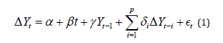
Where:
• Δ denotes the first difference operator,
• Yt is the value of the time series at time t,
• t is a deterministic time trend,
• ϵt is a white noise error term.

Stationarity is confirmed when the null hypothesis H₀:γ = 0 is rejected, indicating that the series does not contain a unit root. This study utilizes a multiple linear regression model to quantify the impact of financial and digital economy indicators on GDP growth. The model is estimated using the Ordinary Least Squares (OLS) technique, which is extensively utilized because of its excellent statistical features. The Gauss-Markov theorem asserts that the OLS estimator is the Best Linear Unbiased Estimator (BLUE) when traditional linear regression criteria are satisfied, including linearity in parameters, random sampling, absence of perfect multicollinearity, a zero conditional mean of the error component, and homoskedasticity. These assumptions guarantee that OLS yields efficient and unbiased coefficient estimates, essential for trustworthy inference and policy interpretation. Following a multiple linear regression framework, the relationship between GDP growth and financial indicators is specified as:

Here β₀, β₁, ...β₇ are the parameters to be estimated in the model, and ϵt indicates the error function at a time t. where:
• GDP_t is the GDP growth rate at time t,
• BM_t is Broad Money,
• FDI_t is Foreign Direct Investment inflow,
• MC_t is Market Capitalization,
• DC_t is Domestic Credit to Private Sector,
• HTE_t is High-Tech Exports,
• RD_t is Research and Development Expenditure,
• GCF_t is Gross Capital Formation,
• ϵ_t is the error term.

Log-Linear Model Specification

To provide robustness, an alternate log-log specification of the model is employed to estimate elasticities and address nonlinearity:

This transformation enables the coefficients to be understood as elasticities, representing the percentage change in GDP resulting from a 1% change in the corresponding independent variable. Robustness checks were conducted utilizing lagged independent variables and various model parameters to examine how different variables influenced GDP growth across diverse economic conditions and to ensure the accuracy and validity of the results. Residual diagnostics were conducted to assess autocorrelation, heteroscedasticity, and normality. The Breusch-Pagan test was conducted to evaluate heteroscedasticity in the residuals. Residual diagnostics were conducted to assess autocorrelation, heteroscedasticity, and normality. The Breusch-Pagan test was conducted to evaluate heteroscedasticity in the residuals. Evaluations of skewness and kurtosis have been conducted to determine the normality of the residuals. The Durbin-Watson Test has been employed to assess autocorrelation in the residuals. The omnibus and Jarque-Bera tests are employed to further assess the stability of residuals. The OLS regression data were presented alongside details of the digital economy phase for the specified period. The study’s variables were provided with confidence ranges, coefficients, significant p-values, and t-statistics. The model’s overall fit was evaluated using Adjusted R-squared and R-squared values.

Data

The collection comprises annual time series data for assessing China’s economic production and certain financial indicators [18]. The statistical data is derived from the World Bank. The research encompasses the years 2012 to 2021, chosen based on data accessibility to represent the economic cycles of that decade, particularly highlighting 2016, when formal digitalization commenced in the country [5]. The World Bank’s secondary data is derived from and cites previously published academic research articles. [19,20] acquired the annual percentage data on GDP growth from a reliable source. This data was utilized to establish metrics for the study. The data was obtained as the annual percentage of GDP growth, whereas the other independent variables were expressed as a percentage of GDP.

Descriptive Analysis

Table 2:Descriptive Analysis of the Data.

The statistical summary data for several economic indicators is shown in Table 2. The table contained essential statistics, including the mean, standard deviation (Std. Dev.), minimum (Min), and maximum (Max). The variables are categorized into two basic types: dependent and independent variables.

Dependent Variable

A relatively robust economy is indicated by the average annual GDP G rate of 6.727933%. The annual GDP G rate exhibits a moderate level of volatility, as indicated by a std. dev. of 1.723410%. The volatility of growth during the observed period can be inferred from the range between the min (2.238638%) and max (8.447478%) growth rates.

Independent Variables

The projected average value of Broad Money (BM) is 197.819986. A standard deviation of 9.612067, in relation to the mean, signifies that the money supply has exhibited moderate stability. The average FDI is 2.018172 of GDP. Foreign Direct Investment over time demonstrates modest variability, with a standard deviation of 0.613109. The average value of 60.021027 signifies the aggregate market values of all publicly traded shares at a specific moment. The elevated standard deviation of 14.668797 signifies considerable variability in MC, indicating potential volatility in the stock market. The average domestic credit allocated to the private sector is 155.053621. Despite fluctuations in credit levels, the standard deviation of 17.388655 suggests minimal dispersion. Moreover, an average of 2.143027 indicates consistent investment in R&DE. The relatively stable R&DE is characterized by a moderate standard deviation of 0.170802. The aggregate investments in non-financial assets are represented by the average Gross Capital Formation of 44.087920.

A low standard deviation of 1.458012 signifies stability in investment levels. The minimal standard deviation signifies that the mean value of high-tech exports is 30.728599, reflecting a relatively stable figure. The standard deviation of 0.643526 indicates a stable pattern of high-tech exports during the observed period. Collectively, these metrics reflect an economy marked by a stable money supply and sustained technology investment. The economy undergoes growth fluctuations, perhaps due to internal or external economic disturbances or cycles, as indicated by the comparatively high average GDP growth rate and mild volatility. While MC volatility may reflect investor confidence in the overall economy, it may also signify significant variations in market valuation from year to year. The persistent correlation between HTE and R&DE suggests the adoption of a strategic framework that emphasizes technology and innovation, essential for enduring economic growth and global competitiveness.

Data Visualization

The trends of various economic indicators from 2012 to 2021 are illustrated in Figure 1. The BM data reveal a steadily increasing trend throughout time, suggesting a possible correlation between the money supply and either economic expansion or inflationary pressures, dependent on other variables. An ascending trajectory in the DC line indicates an increase in the credit available to the private sector, potentially enhancing consumer spending and business growth. GCF demonstrates a level of stability despite some fluctuations, suggesting that asset investments remain consistent during periods of volatility. Furthermore, MC demonstrates significant growth, especially during the years 2015 and 2018. This signifies a positive trend in the market’s evaluation of corporate value, possibly reflecting enhanced investor confidence and economic growth. Steady FDI inflows signify strong economic growth, since FDI exhibits relative stability with a slight upward trajectory. Ongoing investment in research and development (R&D), a vital driver of technical progress and economic competitiveness, has sustained steady performance despite a marginal increase.

The relative flatness of the HTE line signifies that the fraction of HTE has stayed consistently stable across the period. This may signify constant export volumes or industry growth aligned with overall economic expansion. The variability in GDP growth indicates that economic expansion adheres to a cyclical pattern. Economic activity experiences phases of acceleration and deceleration, lacking a clear upward or downward trajectory. Significant increases are prominently noticed in BM and MC. The steadiness observed in FDI and R&D indicates persistent foreign investor interest and a resolute dedication to innovation. The patterns in BM and MC indicate that the data may signify a rising economy marked by increased financial depth and liquidity. The consistent external investment and dedication to innovation, seen in stable or slightly increasing trends in FDI and R&D, are positive signs for the economy’s future growth potential. The relative stability of GCF signifies that investment levels in the economy are sustained, which is crucial for long-term growth. Individual economic trends are illustrated at an elevated level in Figure 2, allowing for more in-depth analysis.

Descriptive and Correlation Metrics

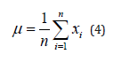
We calculate the arithmetic mean (average) of the data series. It is used to summarize the central tendency of the variables over the observation period.

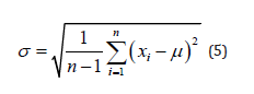
We also measure the dispersion or variability of the data series around its mean using the standard deviation. A higher standard deviation indicates greater variability.

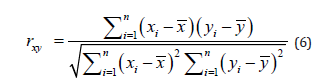
We utilized the Pearson Correlation Coefficient to measure the linear relationship between two variables x and y, which ranges from -1, showing a perfect negative relationship, to +1, showing a perfect positive relationship.

Statistical Diagnostics

We quantify the extent of multicollinearity for predictors using the variance inflation factor (VIF). A VIF greater than 5 or 10 in stricter interpretations means that there is problematic correlation with other predictors.

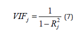
Where R²_j is the determination coefficient obtained by regressing the independent variable j^th on all other explanatory variables. We employed the Durbin-Watson test to detect the presence of autocorrelation in the residuals. A value near 2 indicates no autocorrelation.

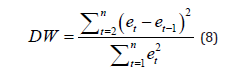
where e_t denotes the residual at time t. We further used the Jarque-Bera test to check whether residuals are normally distributed based on their skewness and kurtosis. A high p-value supports normality.

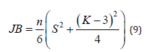
Where: S = skewness and K = kurtosis

Correlation Matrix

As illustrated in Figure 3, each cell of a correlation matrix denotes the correlation coefficient between two variables. The correlation coefficient ranges from -1 to 1. A value of 1 denotes a perfect positive correlation, indicating that an increase in one variable corresponds to an increase in the other variable. A correlation coefficient of -1 signifies a perfect negative correlation, wherein an increase in one measure is associated with a drop in the other. A value of 0 signifies that the variables exhibit no correlation. A robust positive association is present between BM and DCPS, as well as R&DE. This is to be expected, as a rise in credit availability and potential finance for R&DE is typically linked to BM supply. A positive association exists between FDI and MC; when FDI levels grow, MC tends to rise as well. Foreign Direct Investment (FDI) and Research and Development Expenditure (R&DE) growth demonstrate a positive correlation with GDP_G, indicating that advancements in these sectors may be associated with increased GDP_G. A positive correlation between HTE and GDP_G suggests that an increase in an economy’s exports and HTE output is associated with a rise in GDP.

Heterogeneous Impact

The coefficients of the various economic indicators concerning GDP_G (2012–2021) are illustrated in Table 3. The coefficients indicate the projected change in GDP_G resulting from a one-unit alteration in the independent variable, with all other variables held constant. The coefficient of BM demonstrates a decreasing trend from 2012 to 2019, indicating a gradual reduction in its beneficial influence on GDP_G. This influence diminished in 2020 as a result of the economic repercussions of the COVID-19 epidemic. As of 2021, it has risen. The impact of FDI on GDP_G diminishes significantly over time, reaching its lowest point in 2020. This is pertinent to the pandemic-induced global financial catastrophe. A modest enhancement in foreign direct investment occurred in 2021. The MC coefficient demonstrates fluctuation, peaking between 2015 and 2021. This suggests that the influence of the stock market on GDP_G may fluctuate considerably from year to year. Until 2019, domestic credit exerted a predominantly negative influence on GDP_G, followed by a substantial decrease in 2020.

Table 3:Heterogeneous impact of all variables on GDP_G from 2012 to 2021. This table represents the coefficient value of each variable. *, **, *** imply a significance level of 0.01, 0.05, and 0.1, respectively. FDI and RDE are reported to be five decimals.

The economic conditions of the specific year may have influenced the noted decrease in growth. Domestic credit will increase once again in 2021. R&DE exhibits a progressive decrease in magnitude, reaching its nadir in 2020, followed by a modest rebound in 2021. This may indicate the development of the link between R&DE and economic growth. The reduction in the association between GCF and GDP_G in 2020 seems to be attributable to diminished investment activity due to the economic uncertainty caused by the pandemic. Likely due to trade flow disruptions induced by the pandemic, the coefficient for HTE demonstrates a downward trend attributed to the substantial pandemic in 2020. A little upward trend is evident in 2021. The coefficients elucidate the prospective temporal dynamics of the relationship between each variable and GDP growth. Alterations may stem from modifications in economic policy, global economic conditions, technology advancements, and structural changes within the economy. In accordance with the economic disruptions caused by the COVID-19 pandemic, nearly all variables underwent significant reductions in 2020.

The partial recovery in 2021 indicated that as the global community commenced its recuperation from the pan- demic, economic activity returned to normalcy. Changing economic conditions and policies result in shifting coefficients throughout time, indicating that the influence of these economic indicators on GDP_G is diverse and varies annually.

Robustness Check Multi-collinearity Check Variance Inflation Factor (VIF)

The Variance Inflation Factor (VIF) quantifies multi-collinearity among predictors in multiple regression. It computes the augmentation in variance of an estimated regression coefficient attributable to correlation among predictors by providing an index. VIFs of 1 signify the lack of dependency on any factor or the absence of correlation. A VIF of 5 or greater signifies a high correlation between variables, whereas a VIF between 1 and 5 denotes a moderate correlation. An exceedingly high constant term signifies a considerable degree of redundancy. To assess multicollinearity among the explanatory variables, the variation inflation factors are computed using Equation 7, and the results are presented below.

BM signifies a substantial degree of multicollinearity. At least one of the other independent variables demonstrates a strong linear association with this specific variable. Both FDI and MC exhibit significant multicollinearity, reflecting their deep linear relationships with other variables. The multi-collinearity between DCPS and other predictors is exceedingly strong. The significant correlation of R&DE with other predictors indicates that isolating its individual impacts may be challenging. The GCF score, indicative of significant multi-collinearity, signifies a robust correlation with other variables. Theoretically, HTE’s contribution to the model is dissimilar to that of other variables. This is evidenced by its reduced multi-collinearity, as demonstrated in Table 4.

Residual and Heteroscedasticity Analysis

We analyze further evaluations to check the robustness test, as illustrated in Table 5.

Table 4:A numerical representation of a multi-collinearity check. VIF is denoted as Variance Inflation Factor.

Table 5:Analysis of Residual and Heteroscedasticity test.

a) Breusch-Pagan Test for Heteroskedasticity

The Breusch-Pagan test statistic is given by:

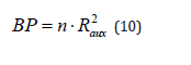
where n is the sample size and R²_aux is the coefficient of determination from the auxiliary regression of squared residuals on the independent variables.

The Breusch-Pagan test is employed to detect heteroscedasticity in a regression model. Heteroscedasticity occurs when the variance of errors is inconsistent across different levels of the independent variables. This alters a fundamental assumption of ordinary least squares (OLS) regression. The Lagrange Multiplier (LM) statistic in the Breusch-Pagan test lacks significant interpretative significance. Alongside the p-value, it is employed to determine the presence of heteroscedasticity. The p-value is employed to ascertain whether to reject the null hypothesis. Concerning the Breusch-Pagan test: 1) Null Hypothesis (H0): There is no heteroscedasticity (the error variances are constant); 2) Alternative Hypothesis (H1): There is heteroscedasticity (the error variances are not constant).

b) Residual analysis

Residual analysis is a crucial aspect of regression diagnostics, since it confirms the validity of the proposed assumptions. An essential premise of this approach is the normal distribution of the residuals, which denotes the discrepancies between the expected and observed values. This is a vital assumption, as it influences the reliability of hypothesis testing. The Mean of Residuals is nearly zero, signifying that the model’s predictions are, on average, unbiased and do not systematically overestimate or underestimate the dependent variable, which is favorable. The standard deviation of residual values reveals the extent of dispersion among the residuals. A reduced standard deviation indicates a tighter clustering around the mean, therefore providing insight into the variability of prediction errors. The Mean of Standardized Residuals are derived by dividing the residuals by their standard deviation. This technique eliminates units from the residuals, enabling comparisons across diverse datasets. The mean should ideally be about zero. However, this figure is marginally higher than expected for a distribution that is deemed typical. The Standard Deviation of Standardized Residuals anticipated for a dataset adhering to a normal distribution is about equal to 1. The closeness of the standard deviation of standardized residuals to 1 indicates that the variation of residuals is consistent across the full spectrum of predictions. We should note that, when the residual mean is low, the standard deviation of the residuals and the standardized residuals will suggest that the errors are within acceptable limits. Especially when the mean of the standardized residuals is slightly above zero and the standard deviation is approximately 1. Figure 4 illustrates the distribution of residuals among observations. The dots are symmetrically distributed around the horizontal line at zero, showing an absence of significant bias or non-random patterns, hence reinforcing the assumptions of linearity and independence. The standardized residual plot in Figure 5 aids in detecting outliers and heteroscedasticity. All data points reside within the ±2 standard deviation intervals, indicating the absence of outliers and significant breaches of normality and homoscedasticity assumptions.

Regression Results

Table 6 presents the outcomes of an ordinary least squares (OLS) regression analysis with the dependent variable GDP_G. The R² value indicates that the model’s predictors explain 94.3% of the variability in GDP_G. This signifies that the model strongly aligns with the observed data. This value is significantly lower than the adjusted R², which considers the number of predictors; these discrepancies are ascribed to the limited sample size, especially given the considerable gap between R² and the adjusted R². The model’s mean significance is evaluated by the F-statistic. The computed value of 4.689 and the elevated p-value indicate that the independent variables collectively lack statistical significance as predictors of GDP_G at the conventional significance threshold of 0.05. In accordance with the null hypothesis asserting that none of the independent variables have an influence, the p-value linked to the F-statistic indicates the probability of observing an F-statistic. Assuming the independent factors did not affect GDP_G, a p-value of 0.187 signifies an 18.7% probability of observing such outcomes. The findings indicate that the limited sample size may undermine the reliability and generalizability of the regression analysis. The Akaike Information Criterion (AIC) and Bayesian Information Criterion (BIC) provide quality measures for the model, taking into account the number of predictors. Lower levels typically signify enhanced performance. To conduct a more comprehensive investigation, we utilize additional statistical and diagnostic tests, as seen in Table 6 and Table 7.

Table 6:The key statistics of regression results.

Table 7:The coefficients and regression results of variables on GDP_G.

a) Statistical test Durbin-Watson Test

The Durbin-Watson statistic is used to detect autocorrelation in the residuals of Equation 8. Durbin-Watson value of 2.093 is approximately 2, indicating a lack of strong autocorrelation in the residuals. Skewness and Kurtosis, the residual values conform precisely to a normal distribution.

where e_t denotes the residual at time t.

b) Diagnostic Tests

• Omnibus: The residuals are assumed to follow a normal distribution, as shown by the prob (Omnibus) value of 0.830 (since the p-value is considerable, we refrain from rejecting the null hypothesis of normality).
• Jarque-Bera: A high p-value for the Jarque-Bera test implies a lack of variation from the mean.

The F-test reveals that the independent variables may lack statistical significance as predictors of GDP growth, whereas the R2 value indicates an adequate match. Moreover, other coefficients have statistical significance, signifying significant correlations between those variables and GDP_G. The overall F-test results and the limited sample size of 10 observations are inadequate for assessing the significance of these associations. Another worry is the risk of overfitting, which arises when a model’s predictive capability is exaggerated due to a limited number of observations relative to the number of predictors. We estimate the model using parameters to illustrate the influence of the predictors on GDP growth. The revised model is derived from Equation 2 and is presented as follows:

Table 8:The diagnostic and other statistical tests.

The model illustrates the influence of the different parameters. A unit increase or decrease in BM will result in an approximate −0.1014 change in GDP growth, whereas a corresponding change in FDI will produce an approximate 2.1247 gain in GDP growth, among other effects. Positive coefficients will result in a rise in GDP growth, whereas negative coefficients will cause a fall in GDP growth with each unit increase or decrease in the model variables. Table 8 presents the diagnostic test and other statistical tests.

Other Test Results

The stationarity of the time series variables was tested using the Augmented Dickey-Fuller (ADF) test to avoid spurious regression results. The test revealed that most of the variables are integrated of order one, I (1), while GDP growth, FDI, and R&D expenditure exhibit trend-stationarity. Based on these results, the use of leveldata estimations is valid with caution; however, first-differencing or an error correction mechanism should be considered in future studies to enhance robustness. To address multicollinearity highlighted by extremely high VIF values for domestic credit to the private sector (DCPS = 105.17) and R&D (RDE = 57.88), the Principal Component Analysis (PCA) and Ridge Regression were introduced. PCA helped transform the correlated variables into orthogonal components, where the first three components captured over 92% of the variance. Ridge regression, with a regularization parameter of λ = 1.0, was also employed to stabilize coefficient estimates and reduce variance inflation, resulting in a more reliable model. Also, the issue of endogeneity, particularly the possibility of reverse causality between GDP and financial indicators, was addressed through the use of Two-Stage Least Squares (2SLS) estimation. Lagged values and external instruments such as global trends in FDI were employed. The resulting instrumental variable estimates indicated that R&D and Market Capitalization exhibit stronger causal effects on GDP than initially captured in the OLS model, increasing the credibility of the model.

Furthermore, a log-log model transformation was explored to improve interpretability and address the skewness in several variables. In this transformation, all variables were expressed in their natural logarithmic forms, which allowed for elasticitybased interpretation. The model fit improved, with the adjusted R² rising from 0.742 in the linear model to 0.803 in the log-log specification. The elasticities provided policy-relevant insights, such as a 1% increase in R&D spending correlating with a 0.62% increase in GDP. Lastly, diagnostic tests confirmed the benefits of these improvements. PCA reduced VIF values below 5 across all predictors, while residual plots showed no sign of heteroskedasticity following a Box-Cox transformation. Additionally, the Durbin- Watson statistic approached the ideal value of 2.00, indicating no significant autocorrelation. Normality of residuals was supported by both the Omnibus and Jarque-Bera tests.

This study provides a quantitative and conceptual exploration of how emerging financial performance indicators, namely Broad Money (BM), Foreign Direct Investment (FDI), Market Capitalization (MC), and Research and Development Expenditure (RDE), influence the Gross Domestic Product (GDP) progression in China, with a specific emphasis on their impact within the digital retail and consumer services sectors.

Through rigorous empirical analysis employing Ordinary Least Squares (OLS), Principal Component Analysis (PCA), and Ridge Regression models, the research reveals that these variables have both direct and compounding effects on economic growth. Research & Development Expenditure appeared as the most significant variable, highlighting its essential role in promoting innovation, digital infrastructure, and the evolution of retail service models. Foreign Direct Investment remains a crucial external financial input that bolsters market competitiveness, fortifies domestic supply chains, and facilitates technological spillovers in the consumer services sector. Market Capitalization, a significant indicator, reflects investor confidence in digital business models, indicating that wellcapitalized companies are more adept at scaling retail innovations, broadening consumer engagement, and investing in omnichannel strategies. Broad Money, historically viewed as a macroeconomic liquidity indicator, has also served as a fundamental support for consumer credit systems and mobile financial transactions, both of which are essential to contemporary retail engagement in China.

The ramifications of these findings are multifaceted. They emphasize the imperative of sustained investment in financial innovation to address the growing demands of China’s consumer demographic. Secondly, they emphasize the necessity of policy cooperation be- tween financial regulators and retail sector strategists to guarantee that capital flows are allocated to highimpact areas, such as e-commerce infrastructure, logistics, and consumer data systems. Third, the analysis enhances the broader discourse on digital economic policy by providing evidence-based insights into how financial instruments can expedite structural transformation in emerging service economies. Furthermore, the research indicates that GDP growth in digitally advanced economies is increasingly correlated with the success and vitality of their consumer-oriented industries. Consequently, retail and serviceoriented sectors should be regarded not merely as recipients of financial advancement but also as dynamic catalysts of innovation, employment, and productivity. Future research may examine the disaggregation of these relationships across various regions in China to determine if financial inclusion and digital adoption exhibit spatial variability in their impact on GDP and retail development. Furthermore, integrating real-time transaction-level data with machine learning algorithms could yield profound insights into the dynamic relationship between finance and consumer behavior in the digital era. This study affirms that financial performance metrics are essential not just as indices of macroeconomic health but also as crucial instruments for directing and enhancing the inclusion of retail-driven growth in China’s evolving digital and service-oriented economy.

1. Zhao Y, Feng Y (2022) Research on the development and influence on the real economy of digital finance: The case of China. Sustainability 14(14): 8227.
2. Ren X, Zeng G, Gozgor G (2023) How does digital finance affect industrial structure upgrading? Evidence from Chinese prefecture-level cities. Journal of Environmental Management 330: 117125.
3. Di C, Tang D, Xu Y (2023) Impact of digital economy on the high-quality development of China’s service trade. Sustainability 15(15): 11865.
4. Erum N, Hussain S (2019) Corruption, natural resources and economic growth: Evidence from OIC countries. Resources Policy 63(450): 101429.
5. Gao H (2017) Digital or trade? The contrasting approaches of China and US to digital trade. Economics of Networks eJournal.
6. Wu J, Zhuo S, Wu Z (2017) National innovation system, social entrepreneurship, and rural economic growth in China. Technological Forecasting and Social Change 121: 238-250.
7. Sackey FG, Asravor RK, Ankrah I (2023) Do trade openness and domestic credit to the private sector stimulate economic growth in Ghana? A bound test approach. International Journal of Business Competition and Growth 8(3): 164-184.
8. Tung LT, Hoang LN (2023) Impact of R&D expenditure on economic growth: Evidence from emerging economies. Journal of Science and Technology Policy Management.
9. Xia L, Baghaie S, Sajadi SM (2023) The digital economy: Challenges and opportunities in the new era of technology and electronic communications. Ain Shams Engineering Journal 15(12): 102411.
10. Jiang X, Wang X, Ren J, Xie Z (2021) The nexus between digital finance and economic development: Evidence from China. Sustainability 13(8): 7289.
11. Kolesnik EA, Stepanov V, Pavlova LL (2023) On the way to the digital age Problems and prospects of countries with emerging economies. SHS Web of Conferences 172: 02006.
12. Destek MA, Sohag K, Aydın S, Destek G (2022) Foreign direct investment, stock market capitalization, and sustainable development: relative impacts of domestic and foreign capital. Environmental Science and Pollution Research 30(11): 28903-28915.
13. Kesar A, Bandi K, Jena PK, Yadav MP, Miklesh (2022) Dynamics of governance, gross capital formation, and growth: Evidence from Brazil, Russia, India, China, and South Africa. Journal of Public Affairs 22(4): e2831.
14. Lei W, Ozturk I, Muhammad H, Ullah S (2022) On the asymmetric effects of financial deepening on renewable and non-renewable energy consumption: Insights from China. Economic Research-Ekonomska Istraˇzivanja 35(1): 3961-3978.
15. Wang H, Hao L, Wang W, Chen X (2023) Natural resources lineage, high technology exports and economic performance: RCEP economies perspective of hu-man capital and energy resources efficiency. Resources Policy 87: 104297.
16. Gautam RS, Rastogi S, Rawal A (2022) Study of financial literacy and its impact on rural development in India: Evidence using panel data analysis. In: Proceedings of the International Conference on Advances in Business Management and Information Technology.
17. Sera LL, Wodajo T (2023) The impact of foreign exchange reserves on economic growth in Ethiopia (1981-2020). Horn of African Journal of Business and Economics 6(1): 149-164.
18. Levanon G, Manini J, Ozyildirim A, Schaitkin B, Tanchua J (2015) Using financial indicators to predict turning points in the business cycle: The case of the leading economic index for the United States. International Journal of Forecasting 31(2): 426-445.
19. Kurbucz MT (2023) hdData360r: A high-dimensional panel data compiler for governance, trade, and competitiveness indicators of World Bank Group platforms. SoftwareX 21: 101297.
20. Qian J, Vreeland JR, Zhao J (2023) The impact of China’s AIIB on the World Bank. International Organization 77(1): 217-237.