Results of Hubble’s Law using the ROR Methodology

There are a large number of natural and even social phenomena in nature, whose occurrence, evolution and final result depend on several independent variables. Even though all these variables intervene in the phenomenon, some are more important than others and even the interrelation between them plays a very important role. The intervention of several independent variables makes the prediction of the occurrence of a natural phenomenon difficult to quantify. Predictive techniques have been developed both in the study of natural phenomena and in social phenomena, each with its scope and limitations.

Currently there are several methods to predict the occurrence of some phenomenon or result, which are included in the predictive analysis (Espino, 2017 [1]). Predictive analytics is a subdiscipline of data analysis that uses statistical techniques, such as machine learning or data “mining,” to develop models that predict future events or behaviors. These predictive models allow you to take advantage of behavior patterns found in current and historical data to identify risks. This type of analysis is based on the identification of relationships between variables in past events, in order to later exploit these relationships and predict possible results in future situations. Doing this is not easy since it must be taken into account that the precision of the results obtained depends a lot on how the data analysis has been carried out, as well as on the quality of the assumptions.

On the trivial level, it might seem that predictive analytics is the same as forecasting (which makes predictions at a macroscopic level), but no, it’s something else entirely. In a crude example, while a forecast can predict how many hurricanes may form in a year, predictive analytics can indicate what intensity and what time of year they are most likely to form, and even where. Therefore, to carry out predictive analysis it is essential to have a large amount of data, both current and past, in order to establish behavior patterns and thus induce knowledge. In the example above, there is more probability of prediction if you also consider variations in regional and global temperature, wind direction, changes and sources of change in pressures etc. This process is done thanks to computational learning. Computers can “learn” autonomously and thus develop new knowledge and capabilities, for this it is necessary to have large databases and predictive analysis tools.

There are currently several techniques applicable to predictive analysis;

i) regression, which includes linear, non-linear, and multivariable adaptive regression; support vectors,

ii) computational learning, which includes neural networks, Naïve Bayes and K-nearest neighbors. One of these tools is the Regressive Objective Regression method that we will explain briefly later. Various applications are included in the bibliography, and the idea is to extend this type of analysis to phenomena in the context of the Zacatecas region. In this new application we will see how Hubble’s law can be obtained using the ROR methodology.

The data for the study were taken from Topic 5,

https://webs.ucm.es/info/Astrof/POPIA/asignaturas/ana_ dat_est/temario.html and own elaboration since it is impossible to copy the pdf database.

Regression analysis is the most widely used statistical technique to investigate or estimate the relationship between dependent variables and a set of independent explanatory variables. In our environment, the ROR methodology has allowed mathematical modeling

a. the larval densities of mosquitoes (Oses, et al. 2018 [2], Fimia, et al. 2018 [3], Oses, et al. 2014 [4]),

b. the population dynamics of mollusks,

c. the modeling of infectious entities of different etiologies, such as HIV/AIDS, Cholera, Influenza, Acute Respiratory Infections (ARI), Covid-19, Acute Bronchial Asthma Crisis (CAAB), Fasciolosis, Angiostrongylosis and even,

d. in the estimation of the longitude and area of the universe, (Oses, et al. 2015 [5], Oses R 2022 [6]) monthly forecast of precipitations and extreme temperatures (Oses, et al. 2018 [7]),

e. forecast of meteorological disturbances (cold fronts, and hurricanes, latitude prediction and length of earthquakes (Oses, et al. 2018 [8]) search for information in white noises (Oses, et al. 2017 [9]) modeling of the Equivalent Effective Temperature (TEE) (Oses et al, 2016 [10]) and Atmospheric Pressure (PA),

f. up to the electricity consumption of a municipality), and more recently in the COVID-19 pandemic (Fimia, et al. 2022 [11], Oses, et al. 2022 [12]).

Using Classical Regression, Hubble’s Law can be obtained in two ways:

1^st….V = H*D, where V is the speed of the Galaxies and D, the distance between them, therefore H is the Hubble constant that is measured in Mpc^-1km/sec, or

2^nd…D = 1/H V, in this article this second option will be used and there will be an approximation of the Law according to the Classical Regression and another using the Regressive Objective Regression, ROR.

Next, Huble’s law for Classical Regression, according to the second formula.

In Table 1, you can see the calculation of Huble’s Law by the traditional method, the corrected R square is 0.878 with a typical error of 0.3893096, the Durbin Watson is close to 1, so more variables can be added in the model.

The Analysis of Variance (Table 2) shows a Fisher’s F of 173.458 significant at 100%.

In Table 3 the traditional model of Huble’s Law of D=1/ H*V.

Table 1: Summary of the Model^c,d.

Table 2: ANOVA^c,d.

Table 3: Coefficients^a,b.

Since D = 0.001 V, therefore clearing we obtain the classic Hubble’s Law, that is: V= 1000 D, so classically the Hubble constant is estimated as 1000 Mpc-1km/sec, according to the second form.

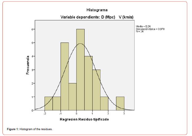
Figure 1 shows the Histogram of the residuals with a mean of 0.24 and a standard deviation of 0.970.

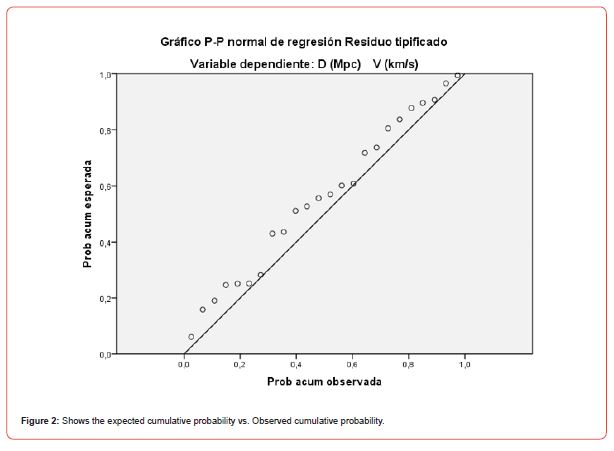
Figure 2 shows the expected cumulative probability vs. Observed cumulative probability.

Next, the result of the residuals. Table 4.

In the case of the ROR methodology (Table 5), a corrected R of 0.996 is obtained with an error of 0.0805881, and this time the Durbin Watson statistic is close to 2, so there is no correlation in the residuals. It can be seen that the standard error of the estimation is smaller than in the classical case (Table 1).

The Analysis of Variance has a Fisher’s F (Table 6) of 759.202 much higher than the classic F (Table 2), so we can state that the ROR model for Huble’s Law is more probable than the classic one.

The ROR model in question can be seen in Table 7. DS is a sawtooth variable and DI is an inverted sawtooth variable, although they are not significant they provide variance to the model, NoC represents the trend of the process which is significant to the increase, the Galaxies are moving away, Lag1 and Lag2 are the distances returned in 1 and two steps and lag4VKms, is the speed returned in 4 steps, which is 90% significant despite the fact that the coefficient is zero.

Table 4: Statistics on residues b^a,b.

Table 5: Summary of the Model^c,d.

Table 6: ANOVA^c,d.

Table 7: Coefficients^a,b.

The NoC trend, which is the trend of the process, was positive and equal to 0.029, so the distance between the Galaxies is increasing, therefore, clearing V from Table 7, it remains:

V_-4 = (0,041/0)*DS +(0.093/0)*DI -(0.029/0)*NoC -(1.147/0)*D-1 +(0,536/0)*D-2 + D/0……………….(1)

Then, substituting 1/0 for i (See 6), a better formula is obtained to measure the speed of Galaxies as a function of Cristosols and an approximation of the Hubble constant as the coefficient of D, that is, H= i = 1/ 0 and is approximately 1000 or better using the Xiomara constant G [6], in such a way that X2 = H= i, since X=√(i), where H is the Hubble constant taken as equal to i so the formula could be:

V_-4 = (0,04*X²)*DS +(0.093* X²)*DI -(0.029* X²)*NoC -(1.147* X²)*D-1 +(0,536 X²)*D-2 + X²……..(2)

D-1, D-2, D are the distances returned in 1 step, two steps and the distance between the Galaxies

V_-4 is the velocity of the Galaxies returned in 4 steps, whose coefficient is zero (Table 7) and for this reason in the formula that we have just written above (1) all the parameters are divided by zero.

In Table 8, the statistics of the residuals, it can be seen that the mean of the residuals is zero and the standard deviation is 0.0691764, in addition the maximum and minimum of the residuals are smaller than those of the Classical regression (Table 4)

In Figure 3 the Histogram of the residuals with ROR. The mean is 2.33 *10-15, and a standard deviation of 0.858, smaller than in the classical model.

Table 8: Statistics on residuals^a,b.

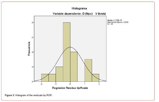
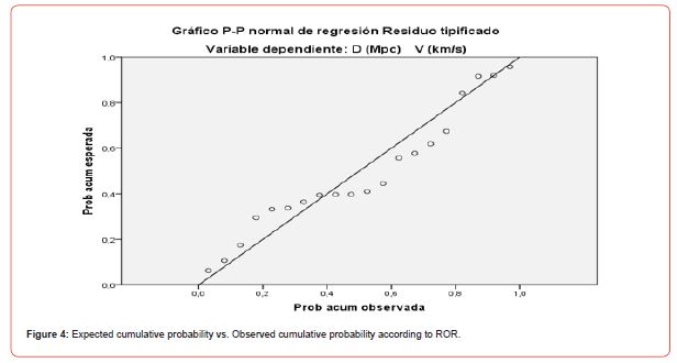
Figure 4 shows the expected cumulative probability vs. Observed cumulative probability according to ROR.

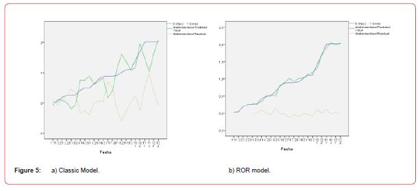
Below (Figure 5) is a plot of the real value against the forecast with its Errors for the classical model and the ROR for the calculation of D.

The best estimate of the Hubble constant is i= 1/0, a Cristosol, classically I is approximately 1000 Mpc-1km/sec assuming that we are approaching the zero moment of the explosion or BIG BANG.

Hubble’s Law is estimated with the Classical Regression as V=1000*D and more exactly with the Regressive Objective Regression as X² = H= i.

ROR Regression measures the Hubble constant more precisely.

None.

No conflict of interest.

1. C Espino Timón (2017) Predictive analysis: techniques and models used and their applications. Thesis, University of Catalonia, Spain.
2. Osés Rodríguez R, Fimia Duarte R, Otero Martín M, Osés Llanes C, Iannacone J, et al. (2018) Incidence of the Annual Rhythm on Some Climatic Variables in Culicidae Larval Populations: Forecast for the 2018 Cyclonic Season in Villa Clara, Cuba. The Biologist (Lima), 16, Jul-Dec, Special Supplement 2. ISSN Printed version: 1816-0719; ISSN Online Version: 1994-9073; ISSN CD-ROM version: 1994-9081. indexed/indexed in: DOAJ-Directory of Open Access Journal, Latindex, Sherpa Romeo, Thomson Reuters-Web of Knowledge (ISI)-Zoological Record, Cite Factor-Academic Scientific Journal. Grupo 2.
3. Fimia Duarte R, Osés Rodríguez R, Iannacone J, Armiñana García R, Roig Boffill BV, et al. (2018) Mathematical Modeling as a Function of Mosquito Focality (Diptera: Culicidae) and Atmospheric Pressure in Villa Clara, Through Regressive Objective Regression. The Biologist (Lima), 16, Jul-Dec, Special Supplement 2. ISSN Printed version: 1816-0719; ISSN Online Version: 1994-9073; ISSN CD-ROM version: 1994-9081. indexed/indexed in: DOAJ-Directory of Open Access Journal, Latindex, Sherpa Romeo, Thomson Reuters-Web of Knowledge (ISI)-Zoological Record, Cite Factor-Academic Scientific Journal. Grupo 2.
4. Osés RR, Fimia DR, Saura GG, Otero MM, Jiménez LF (2014) Modeling of the total larval density of mosquitoes (Diptera: Culicidae) using three models in the province of Villa Clara, Cuba. REDVET 15 (8).
5. Ricardo Osés Rodríguez, Rigoberto Fimia Duarte, Lisvette Cruz Camacho (2015) Simple Model to Estimate Longitude and Area of Universe. Open Access Library Journal 02(03): 1-4.
6. Ricardo Osés Rodríguez (2022) Approximation of the Length of the Universe Calculated with the Cristosols Numbers. Journal of Mathematical & Computer Applications. SRC/JMCA-106.
7. Osés Rodríguez R, Otero Martín M, Fimia Duarte R, Osés Llanes C, Burgos Alemán I et al. (2018) Modelación Y Pronóstico Mensual Con 11 Años De Antelación De Las Precipitaciones Y Temperaturas Extremas Para Cuba. The Biologist (Lima), 16, Jul-Dec, Special Supplement 2. ISSN 43 Printed version: 1816-0719; ISSN Online Version: 1994-9073; ISSN CD-ROM version: 1994-9081. Indexed/indexed in: DOAJ-Directory of Open Access Journal, Latindex, Sherpa Romeo, Thomson Reuters-Web of Knowledge (ISI)-Zoological Record, Cite Factor-Academic Scientific Journal. Grupo 2.
8. Osés Rodríguez R, Carmenate Ramírez A, Pedraza Martínez AF, Fimia Duarte R (2018) Prediction of Latitude and Longitude of Earthquakes at Global Level using the Regressive Objective Regression Method. Advances in Theoretical & Computational Physics (Adv Theo Comp Phy) 1(3): 1-5. ISSN: 2639-0108
9. Osés RR, Aldaz CJW, Fimia DR, Segura OJJ, Aldaz CNG, et al. (2017a) The ROR's methodology an it's possibility to find information in a white noise. Int J Curr Res 9(03): 47378-47382.
10. Osés Rodríguez R, Fimia Duarte R, Iannacone Oliver J, Saura González G, Gómez Camacho L, et al. (2016) Modeling of the equivalent effective temperature for the Yabú station and for the total larval density of mosquitoes in Caibarién, Villa Clara province, Cuba. Peruvian Rev of Entomology 51 (1): 1-7. Grupo 2.
11. Rigoberto Fimia Duarte, Jorge Luis Contreras Vidal, David Del Valle Laveaga, Ricardo Osés Rodríguez, Rafael Armiñana García et al. (2021) Study on the Methodology of Regressive Objective Regression According to the New SARS-CoV-2 COVID-19 Pandemic in the Municipality of Santa Clara and Cuba.
12. Ricardo Osés Rodríguez, Rigoberto Fimia Duarte, David del Valle Laveaga, Luis E Jerez Puebla, Claudia Osés Llanes et al. (2022) Methodology of The Objective Regressive Regression in Function of The Prognosis For Deaths, Critical, Severe, Confirmed And New Cases of Covid-19 In Santa Clara Municipality And Cuba.