The Dynamic of Quantum Spin Interacting with Magnetic Field Coupled to a Heat Bath

Introduction

We explore the critical dynamical properties of single bosonic spin variables, subject to constraints derived from the quantum spherical model of a ferromagnet and coupled to an external heat bath. Our work promotes an understanding of nonequilibrium physics in open many-body systems within finite range interactions.

The Model

We consider N continuous spins Si where i = 1,2, …., N. In a 2D-simple cubic lattice of lattice constant 1, the spins interact by nearest neighbor “exchange forces,” moreover we assume that. S_i ∈ (−∞, ∞) . Note that if S_i = ±1 for all i then we have the Ising model. If we require their total length to be proportional to or equal to N, the number of lattice sites is [1]

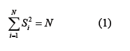
We call Eq(1) the spherical condition. From Eq(1) the spherical model must satisfy the relation

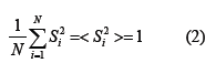
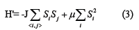
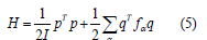
This describes an N-dimensional sphere with radius N1/2, and the points in the sphere are given by Eq(1). In the thermodynamic limit, the microcanonical and grand canonical treatment of condition Eq(2) are equivalents [4]. We choose the grand canonical ensemble by introducing parameterμ , thus the Hamiltonian:

Dynamics introduced into Eq(3) by assigning inertia to the spins. We add kinetic energy term to the Hamiltonian Eq(3)

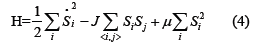
where I is the moment of inertia. Eq(25) represents a d-dimensional system of coupled linear oscillators. This standard classical mechanics problem that can be rewritten as

where α = x, y is the direction in which coupling is taken, and

f is the force matrix constant which is given by

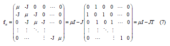
where T is defined by the preceding formula and I is the identity matrix.

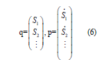
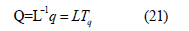
We transform the coordinates as follows:

For the momenta we get

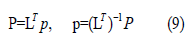
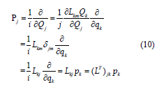
We know that qk = Lkm(Qk). For coordinate Qj the conjugate momentum is (we use the Einstein’s summation convention and chain rule)

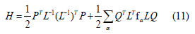
Substitution of the new coordinates and momenta into H yields:

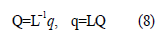
Let us choose L such that it is real and:

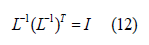
Taking the inverse, it follows that:

And for non-singular L is also follows that:

which means that L is an orthogonal ( and unitary, since it is real) matrix.

We may choose L such that :

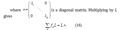
For i^th column of L, denoted by L_i, we have

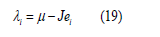
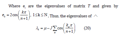
which shows that L_i is an eigenvector of f with eigenvalue λ_i . Thus, to find L we have the eigenvectors and the eigenvalues of f. Substitution of these results into H yields:

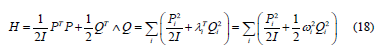
where In other words the transformation q→Q, p→P gave us d uncoupled harmonic oscillators. The frequencies. The frequencies are where λ_i are the eigenvalues of the force matrix constant which is given by Eq(7). Clearly f and T have the same eigenvectors and their respective eigenvalues are related by

The Q_i are called normal coordinates :

Looking at the Hamiltonian in Eq(18) we see the result of quantizing spin S_i

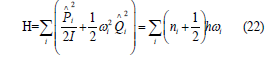
where n_i is the Boson occupation number. Therefore, by analogy we can write the Hamiltonian of a quantum spherical model [2], where the dynamical variables are the spherical spin-operators S_i (at each sitei∈Dwhere

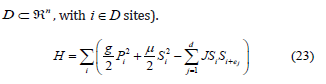
Where g is a coupling constant, μ is the Lagrange multiplier that can be found self-consistently from the constraint 2 i i<Σ S = N > ,and e_j is the j^th cartesian unit vector.

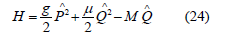
Therefore, the Hamiltonian of a single spherical quantum spin, in an external magnetic field M, reads [3]

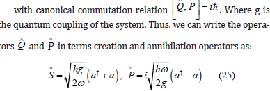
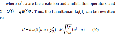
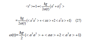
The constraint Eq(2) introduces a relationship between the time dependent frequency and the two-particle-expectation values:

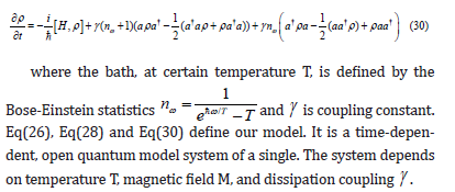
Eq(28) and Eq(26) defines the closed system. Our system of interest is a collection of bosonic spins interacting with a thermal bath. Lindblad’s theory for open quantum systems is the mathematical framework to describe such a system. A coherent quantum (Density matrix) dynamics is formulated by Schrodinger picture

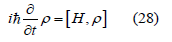
This is Liouville’s equation that describes isolated systems. Coherent dynamics typically last only over short timescales. The coupling to the thermal bath creates dissipation in the quantum systems before the dynamics become dominated by coupling of the open system [3] to its environment, leading to decoherence. Liouville’s equation cannot describe the combination of dissipative and coherent dynamics. To generalize the Liouville Eq(28) to the case of Markovian but unitary evolution, such that ρ = L[ρ ] . Here L generates a finite super operator in the same sense that a Hamiltonian H generates unitary time evolution, which will be called the Lindbladian [3,5]. The Lindblad master equation for an N-dimensional system’s reduced density matrix ρ can

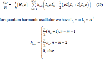
Here nω is the mean number of excitations in the reservoir damping the oscillator and is the decay rate. Thus, we can write Eq(29) as:

Analysis of the Model

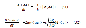
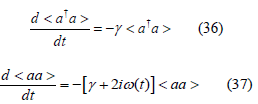
Our goal is to study their time evolution. Therefore, we make use of the Eq(28) and the commutation relation , † i j ij a a  =δ to deduce the closed set of equations of motion for the following averages:

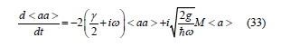
We consider this equation as phenomenological ansatz; thus, by adding the dissipation term −γ < aa > to the equation of motion, we get

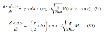
Similarly, we get

In the vanishing Field M = 0 and T = 0 the system described by Eq( 33), Eq(35) and Eq(35) decoupled such that the single particle operators can be treated individually, then we can write:

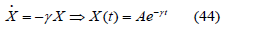
The particle number expectation values decay exponentially

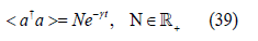
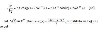
Thus, by using this solution and the spherical constraint Eq(28) the expectation value of the pair annihilation operators obeys the equation

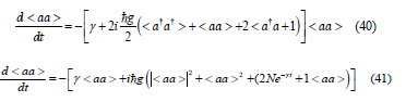
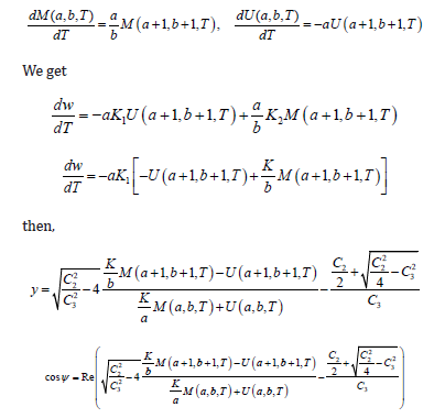
We can separate the amplitude and complex phase by using the substitution < aa >= X (t)e_iψ . Thus, we can rewrite Eq(41) as

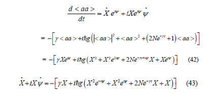
Equating the real parts yields

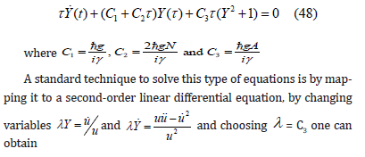
where A is real constant. The imaginary parts yield

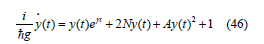
We will make a change of independent variable of the form (change the time scale according to) τ = e^{−γ t} , Y(τ )=y(t) , then

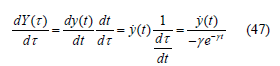
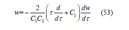
substitute in Eq(24) we get

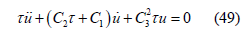
We can simplify Eq(49) to a standard hyper geometric equation by using the substitution u(τ ) = e^−κτω(τ ) , where κ is constant chosen to reduce to the differential equation to the desire form. We get

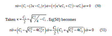
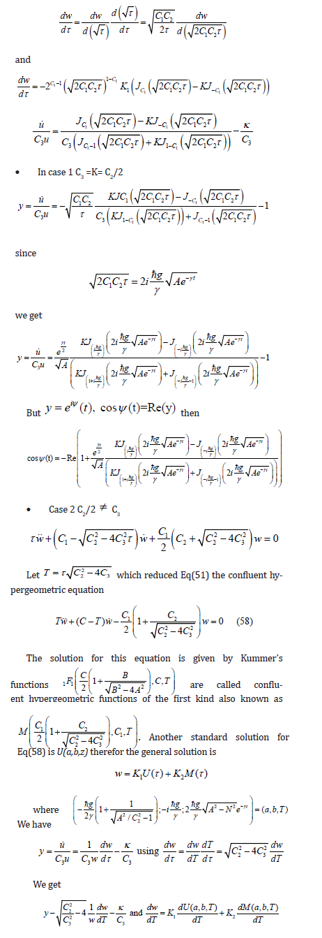
This is a hypergeometric equation that has two distinguish cases [6,7],

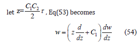
C₂/2 = C3 then Eq(51) turn into

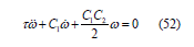
We can rewrite Eq(52) as

Eq(54) is the confluent hypergeometric limit functions and the solution is given by,

When α is not positive integer the substitution

gives linearly independent solution

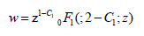
therefore, the general solution is

The confluent hypergeometric limit functions are closely related to Bessel functions. The relationship is

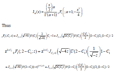
Γ (C₁) and Γ (2-C₁) can be absorbed in the integration constants K₁ and K₂ respectively, and Eq(55) becomes therefore the general solution is

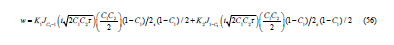
We have used the substitution u=e_−κτ w

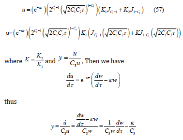
To calculate ω we make use of the Bessel function recurrence relations

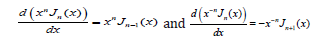
we can write,

we make use of the recurrence relations

From the analysis above, we see distinct phases of the system originates from the coupling, g and ω(t). The two regions of the disordered phase are further illustrated through the relaxation of the magnetization. Although the stationary magnetization always vanishes in the disordered phase, the approach to this stationary value depends on value of the quantum coupling g. The solutions show that the approach towards to stationary value is monotonous. Some magnetic oscillations are also seen for relaxations within the ordered phase. In the solution of Eq(37) which is

and the time dependent frequency w(t) can be reconstructed from Eq(38). The magnetization

followed from integrating Eq(35).

Conclusion

We investigated a simple bosonic spin model behavior in an external Magnetic field in a heat bath. We implemented the meanfield approximation of the dynamics of a quantum spherical ferromagnetic, It presents a quantum analog of well-established typical examples of fluctuation-induced order. The quantum coupling g plays for quantum phase transitions at T = 0 in d dimensions, a role analogous to the temperature T > 0 in classical phase transitions. These zero-temperature quantum phase transitions are stable under a small thermal perturbation.

Acknowledgement

None.

Conflict of Interest

No conflict of interest.

References

- TH Berlin, M Kac (1952) The spherical model of ferromagnetic. physical review B, Second series 86(6): 821.
- JI Budnick, MP Kawatra (1972) Dynamical Aspects of Critical Phenomena. Gordon and Breach, Science Publishers, Inc.
- Andrew J Daley (2014) Quantum trajectories and open many-body quantum systems. Advances in Physics, pp. 77-149.
- Goran Lindblad (1976) On the Generators of Quantum dynamical semigroups. Commun Math 48: 119-130.
- Vittorio Gorini, Andrzej Kossakowski, ECG Sudarshan (1976) Completely positive dynamical semigroups of N‐level systems. Journal of Mathematical Physics 17: 821.
- ET Whittaker, GN Watson (1943) A course of Modern Analysis, American Edition Cambridge: At the University press.
- Bowman F (1958) Introduction to Bessel Functions. New York.
-
This work is licensed under a Creative Commons Attribution-NonCommercial 4.0 International License.