Seismicity and Water Level change in the Caspian Sea, an Explicit Function Based on Genetic Algorithm

Inland water bodies are highly sensitive to environmental changes in their hinterlands. As the largest lake on the Earth, the Caspian Sea has a number of unique features. Not least of there is the considerable water level fluctuations during the 20th century due to changes in the volume of water in the sea. The water surface area in the Caspian Sea is around 380,000 km² depending on the water level. It washes five different countries along almost 7000 km length of coastline, namely Iran, Turkmenistan, Kazakhstan, Azerbaijan and Russia. It is believed that it is a remnant of the Tethys Ocean that became landlocked about 5.5 M years ago, along with the Aral Sea and the Black Sea [1]. It is a sea with no outlets and no tides. Its salinity is only one third of that of the main oceans (up to 13 g/l), decreasing from the north, where the Volga river flows into the sea, to the south basin and also from the west to the east due to fresh water coming from rivers [2,3]. It is conventional to consider the basin of the Caspian Sea as having three parts [4,5]: a northern part, with water depths of only a few meters; a central part, where the water depth increases in a southerly direction with a maximum depth of 788m; and a southern part wherein the water depth increases to over 1000m. Based on the known bathymetry and depending on the water level, the volume of water in the sea is around 78,200 km3. It measures 1,170 km North-South (between latitudes 36° and 47°) and as much as 470 km East-West (between longitudes 49° and 54°) as shown in Figure (1). As a landlocked body of water, the Caspian Sea level (CSL) is controlled by the interplay of the influx of water from a number of rivers, of which the largest is the Volga, and the outflux due to net evaporation. It is believed that the net volume contribution from seepage either into or out of the sea is negligible [6]. The Caspian Sea water balance has been documented in various publications and generally riverine inflow and evaporation from the sea surface are believed to be the major factors [6,7]. River runoff mostly comes from the Volga River. The Volga River Basin is situated within the Russian Plain and this river drains an area of around 1,380,000 km² with a length of about 3700 km and discharges into the northern part of the Caspian Sea (Figure 1). Its annual discharge has been observed to be varied between 212 and 310 km3 [8] (Figure 1).

The Caspian Sea has experienced considerable fluctuations in its water level during the past century. In 1900, the Caspian Sea level (CSL) was about -25.5m relative to global sea level, and it had fluctuated a little around -26m for the previous three decades. In the 1930s, the CSL began to decline rapidly by around 2m, followed by a longer period ending in 1977 at which time CSL was about -29m. By the year 1995, CSL had largely recovered, increasing to about -26.6m. Subsequently it has slightly fluctuated around -26.5m. These profound water level changes in the Caspian Sea have had several impacts on the region: Changed coastal morphology [5,9] seriously affected many national economy branches [10], and even changed the seismic regime [11]. The last of these effects is similar to the problem of Reservoir Induced Seismicity (RIS) (Figure 2).

RIS was detected for the first time in Lake Mead (Hoover Dam) in the United States in 1940s. After that, around a hundred worldwide cases have been reported by researchers such as Gupta, Beck, Simpson, Kalpan and Chander, Awad and numerous others. Many studies were carried out to achieve a better understanding of correlation between dam site conditions with RIS. It is observed that in some cases, Triggered earthquakes occurred by impounding a small reservoir whereas water filling in some other large reservoirs has been not followed by induced earthquakes. Both the Geological setting and the reservoir characteristics are important factors in assessing potential of sites among which the maximum height of water column has a significant effect. There are a number of reservoirs in which RIS has been observed several years after impounding and the earthquakes that occurred have been even larger, both in number and magnitude, than those shaking the region at the time of initial impoundment. This type of RIS can also be related to the lake level oscillations seen in some sites such as Koyna in India, Lake Mead in United States, and Lake Jocassee together with Monticello reservoir both in South Carolina. In the case of Induced earthquakes, given the gradual accumulation of energy in faults of a region, any change in the stress level will stimulate faults, and act as a catalyst to impact the seismic regime. The b-value parameter (see below and equation 1) of the Gutenberg and Richter equation [12] provides a leading seismic source of information in a region [13,14]. Most b-value investigations result in a correlation between this parameter and the physical properties in an area [13]. For example, spatial variations of b-value demonstrate stress variations in an area [13,15]. Scholz [16] showed that the magnitude of the b-value depends on the stress level. Several highquality seismic catalogues were analysed by Schorlemmer et.al [17]. They found that the highest, lowest, and intermediate amounts of b- value belong to the normal, thrust, and strike-slip faulting types of earthquakes, respectively.

If the Caspian Sea were a reservoir, the change in load represented by a 2.6 m increase in water level amounts to a loading of some 1012 tons, hundreds of times the mass of the biggest dam reservoirs, it would almost certainly have led to a significant development of reservoir induced seismicity. For example, studies conducted by Beck on Lake Oroville appeared to show that the weight induced stresses cannot directly trigger earthquakes. In the case of the Caspian Sea, however, the area is huge, and the dimensions of the sea are more than ten times of the thickness of the crust beneath the Caspian Sea. This can lead to crustal flexure, and bending stress on a scale that man-made reservoirs cannot .Since the Caspian Sea is any way situated in a seismically active region; this could be a convincing argument suggesting that the slightest changes in the stress level of the region could stimulate the faults that have a high potential for triggering earthquakes. A study of seismicity patterns in a region and comparing time-depended anomalous variations in the number and magnitude of earthquakes with water level variations (common in RIS studies) cannot be of any help with the case of the Caspian Sea due to lack of data. There is not a rich set of seismic data in the Caspian Sea region specifically recorded before the year 1970, with which to detect detailed anomalies. Hence; the parameter b of the Gutenberg-Richter equation [12] is explored. After finding a relationship between this parameter and water level changes, Genetic Algorithm and RBF neural network methods are applied to formulate the correlation.

The northern part of the Caspian Sea basin is largely devoid of any seismic activity whereas; the southern part has been surrounded by several intense belts of earthquakes including: Apsheron- Balkan, Kopeh Dagh, Alborz, Talesh, Kura Basin and Greater Caucasus. The middle Caspian basin is the area wherein the south Caspian basin lithosphere is subducting beneath the northern crust causing a high level of seismic activity [18]. Earthquakes in Apsheron-Balkhan belt are deep with a normal focal mechanism. Normal faulting in this belt either depends on bending of the South Caspian lithosphere, like oceanic trenches, or is the result of detachment and breaking of slabs at depths and in the mantle . The Kopeh Dag mountain range separates Iran from the Turan platform. In this seismic belt, earthquakes mostly include right-lateral strike slip faulting with N to NNW direction as well as reverse faulting parallel to the direction of the belt. Northwest continuation of the Kopet Dag belt joins the Cheleken-Balkhan seismic band whose active structure is buried beneath the sediments of an old river delta. The Oxus River once flowed to the Caspian Sea and then diverted northward to enter the Aral Sea. For this reason, earthquakes in this region are considerably deeper (27-31 km) than those in the Kopeh Dag i.e. less than 15 km [19]. The Alborz, a high range of mountains, has been stretched parallel to the southern coastline of the Caspian Sea from ~49°E to ~56°E. This seismically active belt starts from the end of the Talesh Mountains in the northwest of Iran and meets the Kopeh Dag in the east, consisting of many summits among which the highest is Damavend volcano with a height of 5,761 m. Based on Jackson et al.[19], the earthquake depths in the Alborz are less than 15 km. In addition, focal mechanisms of more earthquakes in the Alborz belt indicate reverse faulting or left-lateral strikeslip faulting parallel to the Alborz belt. Although the Talesh belt is the west continuation of the Alborz belt but Mechanisms of earthquakes in these two regions are quite different. Thrust earthquakes with depths of 15-26 km (deeper than Alborz earthquakes) occur in the Talesh zone. These depths match with active faults in the basement of the western sedimentary section of the South Caspian Basin, so they may represent a phenomenon whereby the crystalline basement of the South Caspian Basin is thrust beneath Talesh Mountains [19]. The mechanism of most earthquakes in the eastern Great Caucasus is low angle thrusting on both sides of the mountains. It has been suggested that the Eastern Greater Caucasus is being thrust over the southern edge of the Russian plate and on the southern side, sediments of the Kura Trough are being thrust beneath the Greater Caucasus [19]. Therefore the Caspian Sea region presents earthquakes with a variety of focal mechanisms including lateral faulting, large and small angle thrusting and also normal faulting [20], all of which have the potential to be affected by crustal flexure (Figure 3).

Statistical analysis and b-value calculation

The frequency-magnitude distribution of earthquakes is a statistical relationship which relates the number of earthquakes to their magnitude. This was proposed by Ishimoto and Iida in the east and by Gutenberg & Richter [12] in the west and is given as [13]:

Where, N is the cumulative number of earthquakes with a magnitude of M or larger. The constant a, known as a-value, describes the general level of seismicity over a period of time in a study area. For example, a high a-value indicates high seismicity in a given area. The parameter b, known as b-value, is the slope of equation (1), describing the relative number of large earthquakes to smaller earthquakes. It is conventional that the global average of b-value is approximately one [21] but it has not been extended to some cases of seismicity such as induced seismicity [14] and volcanic areas [17]. The regional variations of b-value are found to correlate with stress level variations. Laboratory experiments suggested a direct correlation between the b-value and material heterogeneity, also an inverse correlation between this parameter and the stress level [16,22] such that the temporal variation of the b-value can be suggested as a component of an earthquake warning system [23]. The b-value can be estimated by maximum-likelihood using following equation:

Wheredenotes the mean magnitude and M^min is the minimum magnitude of the given earthquake sample. 𝑒 is the Euler’s number. The determination of min M^min relies on the magnitude distribution. In most cases, the minimum magnitude of data set is determined by plotting cumulative number of events as a function of magnitude. A shaighr best-fit line is found, and min M^min is the level at which the data fall below the line. A correct estimate of the b-value is dependent on the completeness of the data source [13].Another way for calculation of the 𝑀𝑚𝑖𝑛 is to compute the minimum magnitude of completeness, 𝑀𝑐. By applying the maximum curvature method [13], an overall was computed for the Caspian Sea region and lower events were removed from the catalogue. Finally, a correction of must be applied to the calculation in which Δ𝑀 is the correction factor related to rounding errors. Generally, for ΔM = 0.1, it is possible to set , since earthquake catalogues usually give magnitudes only with two digits.

The data and b-value calculation

The International Institute of Earthquake Engineering and Seismology catalogue (IIEES: www.iiees.ac.ir/) covers the area between 23° to 42° N and 41° to 67° E. The catalogue of the Institute of Geophysics University of Tehran (IGTU: www.ngdir.ir/ earthquake/IGTU.asp) is another of Iran’s internal sources which started to report seismic events in 1996 and covers the study area, but it is not of interest, because it does not provide data for the time period. For the Caspian Sea region, the International Seismicity Center catalogue (ISC: www.isc.ac.uk) catalogue is the best source about the desired timeframe and location. A combination of data from IIEES, IGTU and ISC catalogues cannot help due to some reasons. Firstly, merging catalogues together must, depending on the sources, be carried out carefully. Duplicates and different scales are two main problems in combining the catalogues. If there is an overlap in the region in which the catalogues are defined, it is very probable that they have common earthquakes. For the study period, most of the IIEES records can be found in the ISC catalogue. Secondly, both catalogues have to use the same magnitude scale, but this is not always the case and the magnitudes have to be converted. On the other hand, a combination is often used when the desired information cannot be extracted from analysis of one catalogue alone. The ISC catalogue can provide a reasonable database. Table 1 shows the four corner vertices of the Caspian Sea region in which the catalogue is defined. The created catalogue contains 3,499 events which occurred from 1931 to 2009 in the Caspian Sea region, shown in figure 4 (Table 1) (Figure 4).

Table 1: Four corner vertices of the Caspian Sea region.

To examine the temporal variations of the b-value in the Caspian Sea region, b-values were calculated using ZMAP software in sliding time-windows from the earthquakes listed in the catalogue. In other words, a constant number of events (100) were taken and then the window was shifted by N/a=10 events. “N” is the number of events in the window and “a” is an overlap factor. The parameters N and “a” can be varied to obtain the best or compromise result [14]. The experiments showed that using a high number of events in the window could smooth away some of the differences between different parts of the data (especially very short term variations) and in some cases, when a low number of events were chosen, the time-dependent b-values could not be correctly calculated due to the low time resolution of the earthquakes. Figure (5) shows the variation of b-value and Caspian Sea water level over the period 1970 to 2005 in the South Caspian Basin and surrounding areas (Figure 5).

Genetic algorithm: an overview

A genetic algorithm is a class of adaptive stochastic optimization algorithms involving search and optimization. Genetic algorithms were first used by Holland [24]. Not only does GA provide an alternative method to solving problem but although, consistently outperforms other traditional methods in most of the problems. Many of the real-world problems involve finding optimal parameters, which might be difficult for traditional methods but is easy for GA. GA even has been wrongly regarded as a function optimizer regarding its outstanding performance in optimization. The ideas of Genetic Algorithm (GA) presented by John Holland in the 1960s and then extended by Holland and his students and colleagues at the University of Michigan in the 1960s and 1970s [25]. Genetic Algorithm (GA) is an adaptive heuristic search algorithm based on the evolutionary ideas of natural selection and genetic, widely used to solve optimization problems. The basic concept of GA follows the principles laid down first by Charles Darwin for survival of the fittest. Also, GA represents an intelligent exploitation of a random search within a defined search space to solve an exhausted search problem [26]. The GA searches through a set of “chromosomes”, called population. Each chromosome is a string of “bits” or “real values,” and can be a solution to a given optimization problem. Moreover, the GA requires a fitness function which determines the fitness of a chromosome in a population [27]

To solve a clearly defined optimization problem by GA, following steps are involved [28]:

1. Define the structure of chromosome for the problem.

2. Start with a randomly generation of population of N different chromosomes.

3. Fitness evaluation: Calculate the fitness function F(x) of each chromosome x in the current population.

4. Until generating N offspring reiterate the below steps:

a) Choose two chromosomes from the current population as parents. The probability of selection of a chromosome as a parent is a function that increases according to its fitness. The same chromosome has a chance to be selected more than once to be a parent. In other words, selection method is the selection “with replacement”.

b) Crossover the parents with probability 𝑝c at a point which is randomly selected to create a new pair of offspring. In the case that no crossover is done, exactly copy the current parents to offspring.

c) With mutation probability 𝑝𝑚 , mutate each locus of the two chromosomes in the offspring and put them in the new population.

5. Substitute the new population for current population.

6. If the termination condition is not satisfied go to step 2, otherwise terminate the algorithm.

7. This simple procedure of GA has been utilized to solve many problems with an acceptable precision. In this paper, we use it to approximate the parameters of an explicit function that predict the non-linear correlation between b-value and water level in the Caspian Sea region.

Computing explicit function parameters using GA

Figures 5 showed that there is a non-linear explicit correlation between the b-value and water level in the Caspian Sea region. This correlation is clearly illustrated in Figure 6 which depicts the b-value versus corresponding water level (Figure 6).

Data acquisition mostly deals with many problems, among which the noise is an unavoidable one. To solve this problem, the noise reduction and outlier elimination are two main steps in data processing (Tan, 2006). In this research an RBF neural network (Kuo et al., 2009) is used to smooth the data set and remove its noise. After filtering, the filtered signal showed that the non-linear correlation between b-value and water level can be formulated using a sinusoidal function (figure 7) as following:

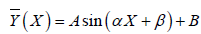
Where the parameters of the function can be computed efficiently using GA [29].

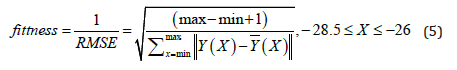
These parameters should be computed such that the sum of squared errors between the desired explicit function, equation (3), and original data set is minimized. This can be explained as following:

Where 𝑌(𝑋) is the original values and Y ( X ) is the approximated values resulting from equation (3). In the experiments, the size of initial population for GA is considered to be 100. The crossover probability, mutation probability, and the maximum number of generations is considered to be 𝑝𝑐 = 0.9, 𝑝𝑚 = 0.02 and 5000 respectively. The range of inputs and outputs for GA are set as the minimum and the maximum values of input variables. To achieve the best value of the parameters a fitness function is defined as the inverse of root mean square errors (RMSE) [29] which should be maximized:

The algorithm utilizes the standard GA operation; singlepoint crossover, bitwise bit-flipping mutation and selection with Roulette Wheel method, and the GA algorithm is repeated until the termination criterion is satisfied [24,25]. Table 2 shows the computed parameters of equation (3) using GA. Also, Figure 7 illustrates the original function and the approximated sinusoidal function. There exist some differences between the approximated and the original values. Since the real data was noisy, these errors are unavoidable and can be ignored. Figure 8 illustrates the estimated b-value for the Caspian Sea region throughout the past century and over a part of 19th century using the approximated function (Table 2).

Table 2: Calculated Parameters of Equation (1) Using GA.

(Figure 7) The history of reservoir induced earthquakes, their common characteristics, and their mechanism of occurrence developed some methods for detecting signs of change in the seismic regime in the Caspian Sea region resulting from the additional loading of the Earth’s crust induced by changes in the water level. It is well-known that, after the start of impounding a reservoir earthquake may begin to occur if there is a potential to trigger seismicity in the dam site hence faults are near to slip. Also, a change in water level in reservoirs may trigger earthquakes even after years or in some cases after decades of initial filling. This suggests that RIS signals might be detected considering the pattern of water level change in the Caspian Sea. But impounding reservoirs triggers seismicity in locations that are already prone to earthquakes. The Caspian Sea Basin, surrounded by several active belts of earthquakes, is a part of the Alpine-Himalayan seismic belt. Morphological and stratigraphically investigations documented in a variety of publications show an active tectonic for the Caspian Sea Basin and surrounding areas and almost all faults of the region can be regarded as active faults. Thus, the effect of loading the crust resulting from a water level change in the Caspian Sea can induce earthquakes in this region which is already prone to seismicity. Considering the available data, the b-value parameter of the Gutenberg-Richter Power Law was selected for examination. This parameter represents the relative occurrence of high and low magnitude earthquakes in a region; a low b-value indicates that the number of large earthquakes is greater than that of small earthquakes and vice versa. The temporal variation of b-value is suggested as an earthquake warning system [23]. It has been found that the b-value decreases with an increase in shear stress or effective stress [14]. The temporal variations of this parameter over the period 1961 to 2005 were computed in the region of the Caspian Sea. The result shows that the b-value had an increasing trend from around 1960 to 1978 demonstrating an inverse correlation between this parameter and water level variations. From around 1978, the trend in variations in b-value was reversed confirming the obtained correlation with Caspian Sea level changes; from 1977 to 1995 the Caspian experienced an increase in its water level. Since the b-value is believed to be inversely correlated with stress level, it is suggested that loading of the crust induced by changes in the Caspian Sea level resulted in an increase in the stress level in the region and with increasing stress the b-value decreased. In the case of a falling water level the unloading of the crust resulted in a decrease in the stress level leading to an increase in b-value. Regarding the available data, only b-values for the period of 1960 onwards could be correctly calculated. To estimate this parameter over the whole period that water levels were instrumentally recorded the correlation was formulated using Genetic Algorithm. The obtained result would calculate b-value as a function of water level. Thus, if the water level data of the Caspian Sea is available, the b-value could be calculated using this method even for a period during which there is not enough seismic data. For this reason, by illustrating the b-value versus corresponding water level, a continuous function was fitted, and the data was smoothed using RBF neural network. Genetic Algorithm (GA) is widely used to solve defined optimization problems with an acceptable precision. The idea of Genetic Algorithm was used to approximate the parameters of an explicit function that estimates the non-linear correlation between b-value and Caspian Sea water level.

The b-value calculation, using related methods [13], for the Caspian Sea region can be correctly done only over the period after the year 1970. Before this year, however; the available set of data is not rich enough. Fortunately, a set of instrumental Caspian Sea water level records is available over the 20th century and the b-value can be estimated throughout the past century using the approximated function.

In Figure 8, the inverse correlation between the Caspian Sea level and the b-value in the region can be seen for a period between 1835 and 2006. There is an up-warping trend from 1936 to 1977. In this period, Caspian Sea level was dramatically declining. It also properly works for the period from 1977 to around 2003. This confirms that the obtained function is correctly works over the period 1936 to 2003. This period is marked with high amplitude changes in the water level. For the rest of the period, from 1837 to 1930 the Caspian Sea did not experience any considerable oscillation in its water level while the approximated function was defined using data related to the high amplitude variations in the Caspian Sea level. In other words, according to the nature of neural networks and GA, predictions can be correctly done on data points which are in the range of those are used for training. It is why this function, which obtained from data belonging to the period of high amplitude variations, namely from 1970 to 2005, is not able to correctly estimate the b-values over the period during which only an amplitude of 0.5m fluctuations can be seen in water level, namely from 1837 to 1930 [30,31] (Figure 8).

Over the past century, the Caspian Sea has experienced considerable fluctuations in its water level. This phenomenon affected the seismicity in the Caspian Sea region, which is highly prone to earthquake, and the b-value of the Gutenberg-Richter Relationship had a non-linear inverse correlation with water level change. It was possible to calculate the b-value only for the period of recent decades due to lack of the recorded seismic data for the years before 1970. This paper contributed to the knowledge about the past seismicity in the Caspian Sea region, for periods preceding the existence of instrumental data, and an explicit sinusoidal function was proposed to predict b-value as a function of water level in the Caspian Sea region using RBF neural network and genetic algorithm, introducing a strong tool to estimate the b-value for all years of the past century. The seismic response of the region to sea level changes was examined even for periods with a lack of data. The experiments showed that the approximated function can be applied to estimate the b-value over the periods during which large amplitude fluctuations occurred in the water level of the Caspian Sea because the function was trained with data related to high amplitude fluctuations.

I must thank Dr. Ali Amiri for his help, discussion, support and helpful suggestions.

No conflict of interest.

1. Boomer I, Grafenstein UV, Guichard F, Bieda S (2005) Modern and Holocene sublittoral ostracod assemblages (Crustacea) from the Caspian Sea: A unique brackish, deep-water environment. Palaeogeography Palaeoclimatology Palaeoecology 225: 173– 186.
2. Kroonenberg SB, Badyukova EM, Storms JEA, Ignatov EI, Kasimov NS (2000) A full sea-level cycle in 65 years: barrier dynamics along Caspian shores. Sedimentary Geology 134(3-4): 257-274.
3. Peeters F, Kipfer R, Achermann D, Hofer M, Aeschbach-Hertig W, et al. (2000) Analysis of deep-water exchange in the Caspian Sea based on environmental tracers. Deep-Sea Research 47: 621-654.
4. Froehlich K, Rozanski K, Povinec P, Oregioni B, Gastaud J (1999) Isotope studies in the Caspian Sea. The Science of the Total Environment 237/238: 419-427.
5. Kaplin PA, Selivanov AO (1995) Recent coastal evolution of the Caspian Sea as a natural model for coastal response to the possible acceleration of global sea-level rise. Marine Geology 124: 161-175.
6. Shiklomanov IA, Georgievski V, Kopaliani ZD (1995) Water balance of the Caspian Sea and reasons of water level rise in the Caspian Sea. UNESCO-IHP-IOC-IAEA Workshop on Sea level rise and the multidisciplinary studies of environmental processes in the Caspian Sea region, Intergovernmental Oceanographic Commission, Workshop Report 108-Supplement, UNESCO, Paris, 1–27.
7. Mansimov MR (1995) Long-standing fluctuation of the level and flooding of the Caspian Sea at the contemporary stage. UNESCO-IHP-IOC-IAEA Workshop on Sea level rise and the multidisciplinary studies of environmental processes in the Caspian Sea region, Intergovernmental Oceanographic Commission, Workshop Report 108-Supplement, UNESCO, Paris pp.48–55.
8. UNESCO/ROSTE (2004) Integrated impact analysis of Volga River Discharge Regulation on Floodplain and Delta Ecosystem.
9. Firoozfar A, Bromhead EN, Dykes AP, Lashteh Neshaei MA (2011) Southern Caspian Sea coasts, morphology, sediment characteristics, and sea level change. Proceedings of 27^th Annual International Conference on Soils, Sediments, Water & Energy, Massachusetts, USA.
10. Kroonenberg SB, Abdurakhmanov GM, Badyukova EN, van der Borg K, Kalashnikov A, et al. (2007) Solar- forced 2600 BP and Little Ice Age Highstands of the Caspian Sea. Quaternary International 173-174: 137-143.
11. Firoozfar A, Bromhead EN, Dykes AP (2012) Caspian Sea level change impacts regional seismicity. Journal of Great Lakes Research 38: 667–672.
12. Gutenberg R, Richter CF (1944) Frequency of earthquakes in California. Bulletin of the Seismological Society of America 34: 185-188.
13. Wiemer S, Wyss M (2002) Mapping spatial variability of the frequency-Magnitude distribution of earthquakes. Advances in Geophysics 45: 259–302.
14. Nuannin P (2006) The potential of b-value variations as earthquake precursors for small and large events, PhD dissertation, Uppsala: Uppsala University, Sweden.
15. Schorlemmer D, Wiemer S, Wyss M (2004) Earthquake statistics at Parkfield: 1.Stationarity of b-values. Journal of Geophysical Research p.109.
16. Scholz CH (1968)The frequency–magnitude relation of micro fracturing in rock and its relation to earthquakes. Bulletin of the Seismological Society of America 58: 399-415.
17. Schorlemmer D, Neri G, Wiemer S, Mostaccio A (2003) Stability and significance tests for b-value anomalies: Example from the Tyrrhenian Sea. Geophysical Research Letters 30(16): 1-3.
18. Priestley K, Baker C, Jackson J (1994) Implications of earthquake Focal mechanism data for the active tectonics of the South Caspian Basin and surrounding regions. Geophysical Journal International 118: 111–141.
19. Jackson JA, Priestley K, Allen M, Berberian M (2002) Active tectonics of the South Caspian Basin. Geophysical Journal International 148: 214-245.
20. Engdahl ER, Jackson JA, Myers SC, Bergman EA, Priestley K (2006) Relocation and assessment of seismicity in the Iran region. Geophysical Journal International 167: 761–778.
21. Oencel AO, Wyss M (2000) The major asperity of the 1999 M7.4 Izmit earthquake, defined by the micro seismicity of the two decades before it. Geophysical Journal International 143: 501- 506.
22. Enescu B, Ito K (2003) Values of b and p: their Variations and Relation to Physical Processes for Earthquakes in Japan. Annuals of Disaster Prevention Research Institute 46B, Kyoto University.
23. Weeks J, Lockner D, Byerlee J (1978) Changes in b-values during movement on cut surfaces in granite. Bulletin of the Seismological Society of America 68: 333-341.
24. Holland JH (1975) Adaptation in Natural and Artificial Systems. University of Michigan Press.
25. Holland JH (1993) Innovation in Complex Adaptive Systems: Some Mathematical Sketches. Santa Fe Institute.
26. Goldberg DA (1989) Genetic algorithms in search, optimization, and machine learning, MA: Addision-Wesley.
27. Gen M, Cheng R (2000) Genetic Algorithms and Engineering Optimization. John Wiley & Sons.
28. Mitchell M (1999) An Introduction to Genetic Algorithms, MIT Press, USA.
29. Lee ZJ (2008) a novel hybrid algorithm for function approximation. Expert Systems with Applications Journal 34: 384–390.
30. Kuo RJ, Hu TL, Chen ZY (2009) Evolutionary Algorithm Based Radial Basis Function Neural Network for Function Approximation. 3rd International Conference on Bioinformatics and Biomedical Engineering 1-4.
31. Tan PN, Steinbach M, Kumar V (2006) Introduction to Data Mining. Addison-Wesley, USA.