Accelerating a Geostatistical Approach to Groundwater Pollution Source Identification with GPU Computing

Pollution source identification (PSI) refers to reconstructing the pollution source locations and releasing histories from observed concentration records [1]. The PSI can be classified into three typical types [2]: namely, finding the release history of a source, finding the location of a source, and recovering the initial distribution of a contaminant plume. As one of the first steps in environmental remediation project, the PSI could be used to making a cost-effective remediation strategy, partitioning the cleanup cost among liable parties [3].

The mathematical and simulation approaches of pollution source identification have been extensively investigated in the past thirty years. The existing mathematical methods could be divided into four major groups, namely optimization, analytical and direct methods as well as probabilistic and geostatistical approaches [4,5]. A probabilistic approach combining Bayesian theory and geostatistical techniques was by Snodgrass and Kitanidis (1997) to estimate the pollution source function [6]. The method is an improvement from some other methods in that the solutions are more general and make no blind assumptions about the nature and structure of the unknown source function. Limitation to this approach is that the location of the potential source must be known a priori [4]. The geostatistical approach has been used to find the source function in a 2D problem [7] to identify the source function in a 3D problem [8] and to find both the source function and location [9]. Some researchers have discussed finding the source release history in a 1D homogeneous aquifer based on the geostatistical approach considering first order reaction [10].

In geostatistical approaches, the researchers usually use Levenberg- Marquart, Gauss-Newton method to find the optimal structural parameters of the geostatistical model [6,9,11]. These methods involve iteration and matrix computation which might lead to high computation cost when the problem is complex. More efficient algorithm [12], surrogate model [13] and parallel computing [14] are usually used to improve the computation efficiency of the simulation model. The parallel computing technique is suitable for largescale matrix and iteration and has been used to solve the PSI problems [15], but the large-scale computation resources are needed in this research. The personal computer could have many graphics processing unit (GPU) cores which could be used in parallel computing. The GPU parallel technique has been used in molecular dynamics and polymer chemistry [16], but the application in the PSI problem is seldom reported.

In this study, we focus on employing the GPU parallel technique to accelerate the geostatistical approach to the PSI problem. Firstly, the geostatistical approach is introduced. Then, we describe how to use the GPU technique to accelerate the PSI problem. Finally, a numerical case is used to show the computational speedups attained through the parallel implementation.

Geostatistical model

The relative between the pollution source release process and the concentration observation could be generalized as [6, 9]:

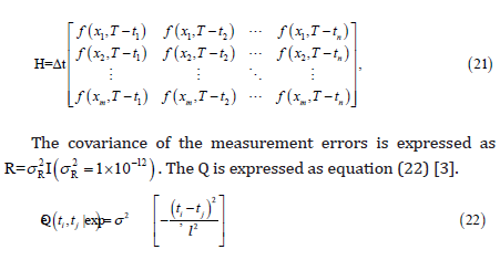
Where z is a m×1 vector of observations, H is a known sensitivity matrix assembled by transfer function [11], s is a n×1 “state vector” obtained from the discretization of the unknown function that we wish to estimate. The measurement error is represented by the vector v which is assumed to have zero mean and known covariance matrix R The expected value and covariance of s could be expressed as equation (2) and (3).

The estimation procedure is divided into two parts [6, 17] (Figure 1). First the optimal structural parameters are found, and then the unknown function is estimated.

The structural parameters are estimated by maximizing the probability of the measurements given :

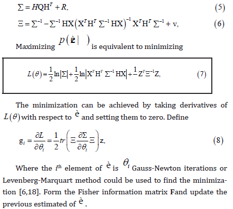
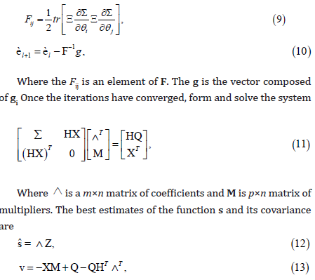
Parallelization of the geostatistical approach

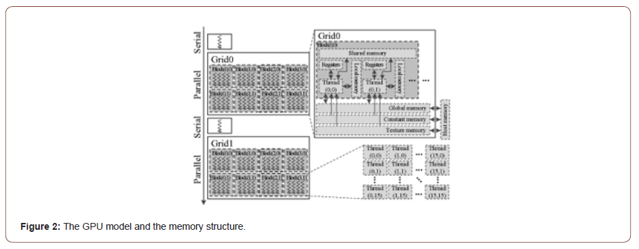
The CPU is the host which execute serial computing and logical operation, and the GPU is the device which execute threading parallel tasks [19]. The GPU model and the memory structure are shown in Figure 2. The function calculated by the GPU is called kernel. The kernel is organized in the form of a thread grid. Each grid consists of several blocks. Each block consists of several threads. The blocks are executed in parallel, and the threads are also executed in parallel. The internal memory of GPU includes shared memory, local memory, and register. The thread also can access the global memory, constant memory, and texture memory. We use Compute Unified Device Architecture (CUDA) and Open-Source Computer Vision Library (OpenCV) to implement the GPU parallelization. Vaidya shows how CUDA allows OpenCV to handle complex processing in computer and machine vision by accessing the power of GPU [20].

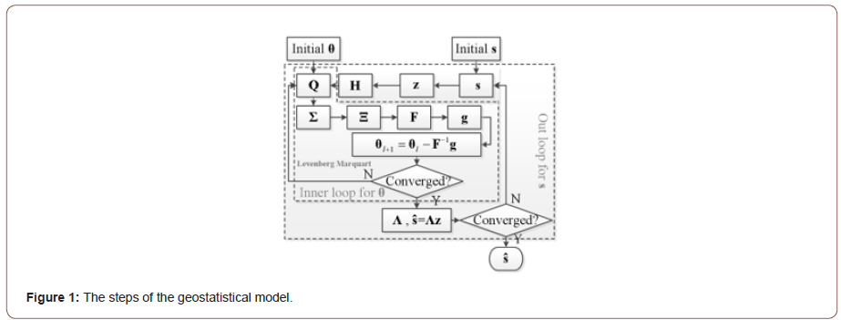
The iteration operation and matrix computation are the main steps to solve the geostatistical model (Figure 1). The initial è and s are input to the inner loop to find the estimated è , then estimated è is input the out loop to evaluate the s When both the out and inner loops are converged, the è and s are found. The operation of è and s estimation cost 90% computing time. So, accelerating the è and s estimation are the key steps to reduce the computing time. Solving linear equations is the main process of the out loop which takes the inner loop result as inputs. The CPU could afford this operation. The inner loop involves a lot of iteration operation and matrix computation. Especially, the Levenberg-Marquart method costs 79% computing time, and finding derivatives of L(θ )costs 13% of the inner loop. The GPU could be used to accelerate the inner loop.

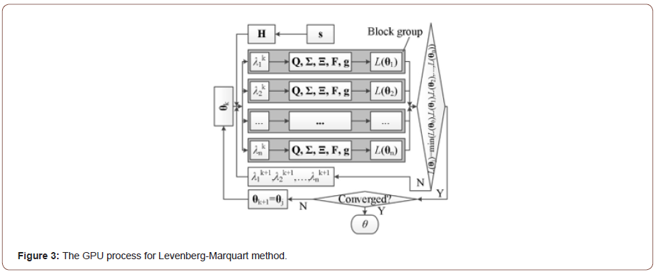
The Levenberg-Marquart method requires that the value of objective function should be decreased after each iteration. The coefficient λ is used to control the search direction of the objective function. The λ is adjusted until the search results meet the requirements that the jth ( ) j L θ corresponding to the jth j λ should be smaller than the ( ) 1 1 th j j Lθ − − . In serial operation, a lot of iteration steps would be conducted to find the λ and è . A parallel Levenberg- Marquardt algorithm [21] is employed to accelerate the operation in this paper. The blocks in a grid of the GPU are divided into several block groups (Figure 3). Each block group conducts all the operation corresponding to aλ . When the operation is converged, the è is found and could be input into the out loop to find the s.

One-dimensional solute transport process case [3] is used to evaluate the method in this paper. It supposes the pollutant transport in a homogeneous aquifer, the actual mean velocity is a constant, the problem could be expressed as [22]:

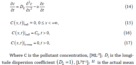
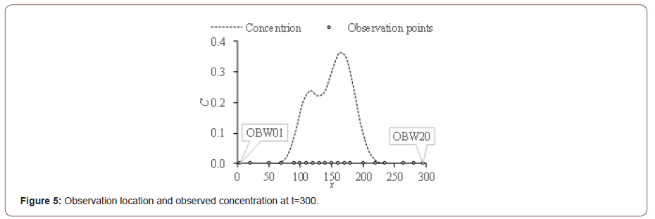
Equation (18) describes the true release history (Figure 4). There are 20 observation points in the direction and the curve of observed concentration z at t=300 is shown in Figure 5. The equation (14) has the solution given by the equation (19) [22].

Experiment environment and the identification result

We use CUDA 8.0 and OpenCV 4.1.0 to implement the GPU parallelization on a Dell Precision M6800 computer assembled with the Intel® Core™ i7-4910MQ CPU @ 2.90GHz, random access memory 32 GB, and a NVIDIA Quadro K4100M GPU.

We obtain the breakthrough curves of each observation points of the numerical case mentioned above (Figure 6). The observation points OBW18~OBW20 are far from the pollution release source, and the breakthrough curves have not reach 1 at t=300. The transfer function curves of these observation points are getting flat when the distance from release source increases (Figure 7). The calculated release history curve is identical to the study [3,7,9,11]. The calculated curve has good agreement with the real release history (Figure 3), their correlation r is 0.998, so the method we proposed could identify the release history. The Euclidean distance de between the up and low bound of the 95% confidence interval is used to evaluate the confidence interval. The de of the identified result is below 6.1, it shows that the uncertainty of the calculated history is small.

Comparison with serial results

We compare the results of GPU parallelization scheme to the serial results. The calculated curve of parallelization scheme has good agreement with the serial result and the real release history (Figure 9). It is difficult to tell the difference between the result of parallelization scheme and the serial scheme from the concentration curves. We use the absolute error and relative error between the result of parallelization scheme and the serial scheme to evaluate the difference. The absolute error falls between -0.015 and 0.015 and fluctuates obviously when the t falls in [110, 220] (Figure 10). But the relative error show low volatility in this interval. When the t does not fall in [110, 220], the concentrations of parallelization scheme and the serial scheme approach to 0, so the difference between them is small. The result of serial scheme acts as very small denominator in relative error. It leads the relative error to appear obviously. When the t falls in [110, 220], the opposite has occurred.

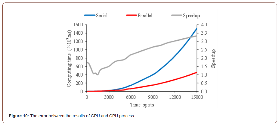
Speedup is the ratio of time consumed by the same task running in single processor system and parallel processor system [23]. If the speedup equal to the number of processors of the parallel computing, the speedup is called linear speedup or ideal speedup. If the time consumed by single processor system is the time corresponding to the most efficient algorithm, the speedup is called absolute speedup. In the geostatistical approach, the iteration and matrix processes are related to the H which is a m×n matrix. The dimensions of the H are decided by the number of observation m and the number of time spots n. The n is far greater than the m in practical problems, so we use n to analyze the speedup. Figure 11 shows the speedup of the result of parallelization scheme and the serial scheme. When the number of time spots is smaller than 5000, the efficiency of parallel process is closed to serial scheme. If the number of time spots increases, the dimension of the H increases which leads to the computation load increase. Then, the advantage of the parallel process appears obvious gradually. The speedup increases from 1 to 3.5 approximately. In study of Cao et al. [21], the speedup of the parallel Levenberg-Marquardt algorithm varies from 1 to 6.39. In this study, the parallel process is used to accelerate the inner loop, while the out loop is dealt with serial scheme. The algorithm could only improve the computing efficiency partially. The algorithm and code of this paper could be tuned to improve the efficiency.

This paper focus on employing the GPU parallel technique to accelerate the geostatistical approach to the PSI problem. Firstly, we introduce the geostatistical approach. Then, we explain how to accelerate the PSI problem with use the GPU technique. Finally, a numerical case is used to analyze the performance of the parallel method. We conclude this work as below:

The method proposed in this paper could identify the release history perfectly in the numerical case.

By applying a parallel scheme, the computing efficiency of geostatistical approach is improved. But the parallel scheme and code of this paper could be improved for more efficiency.

In future research we will analyze the performance of the parallel method considering more complex condition such as the presence of measurements errors of unknow variance, the case of multiple sources and situations in which none of the candidate locations overlaps with the true source.

None.

No conflict of interest.

1. Sun AY, Painter SL, Wittmeyer GW (2006) A constrained robust least squares approach for contaminant source release history identification. Water Rescour Res 42(4): 263-269.
2. Milnes E, Perrochet P (2007) Simultaneous identification of a single pollution point-source location and contamination time under known flow field conditions. Adv Water Resour 30(12): 2439-2446.
3. Skaggs TH, Kabala ZJ (1994) Recovering the release history of a groundwater contaminant. Water Rescour Res 30(1): 71-79.
4. Juliana A, Amvrossios CB (2001) State of the art report on mathematical methods for groundwater pollution source identification. Environ Forensics 2(3): 205-214.
5. Long Y, Li W, Huang J (2012) Advance of optimization methods for identifying groundwater pollution source properties. Appl Mech Mater 178: 603-608.
6. Snodgrass MF, Kitanidis PK (1997) A geostatistical approach to contaminant source identification. Water Rescour Res 33(4): 537-546.
7. Butera I, Tanda MG (2003) A geostatistical approach to recover the release history of groundwater pollutants. Water Rescour Res 39(12): 291-297.
8. Michalak AM, Kitanidis PK (2004) Estimation of historical groundwater contaminant distribution using the adjoint state method applied to geostatistical inverse modeling. Water Rescour Res 40(8): 474-480.
9. Butera I, Tanda MG, Zanini A (2013) Simultaneous identification of the pollutant release history and the source location in groundwater by means of a geostatistical approach. Stoch Env Res Risk A 27: 1269-1280.
10. Long Y, Cui T, Li W, Gai Y (2018) A geostatistical approach to groundwater pollution source identification considering first order reaction. Desalin and Water Treat 123: 35-40.
11. Butera I, Tanda MG, Zanini A (2006) Use of numerical modelling to identify the transfer function and application to the geostatistical procedure in the solution of inverse problems in groundwater. J Inverse Ill-Pose P 14(6): 547-572.
12. Ghafouri HR, Darabi BS (2007) Optimal identification of Ground-Water pollution sources. Int J Civ Eng 5: 144-154.
13. Aarl MM, Guan J, Maslia L (2001) Identification of contaminant source location and release history in aquifers. J Hydrol Eng 6(3): 225-234.
14. Mahinthakumar GK, Sayeed M (2005) Hybrid genetic algorithm – local search methods for solving groundwater source identification inverse problems. J Water Res Pl-Asce 131(1): 45-57.
15. Mirghani BY, Mahinthakumar KG, Tryby ME, Ranjithan RS, Zechman EM (2009) A parallel evolutionary strategy based simulation–optimization approach for solving groundwater source identification problems. Adv Water Resour 32(9): 1373-1385.
16. Energy Minimization Multi-Scale Group of State Key Laboratory of Multiphase Complex Systems (2009) Parallel computing of multiscale discrete simulation based on GPU, China Science Publishing & Media Lid, China.
17. Kitanidis PK (1995) Quasi-linear geostatistical theory for inversing. Water Rescour Res 31(10): 2411-2419.
18. Madsen K, Nielsen HB, Tingleff O (2004) Methods for Non-Linear Least Squares Problems. Informatics and Mathematical Modelling, Technical University of Denmark, Denmark.
19. Zhang S, Chu Y (2009) CUDA of GPU high performance operation. China Water & Power Press, China.
20. Vaidya B (2018) Hands-On GPU-Accelerated computer vision with OpenCV and CUDA[M]. Packt Publishing Ltd, UK.
21. Cao J, Novstrup KA, Goyal A, Midkiff SP, Caruthers JM (2009) A parallel Levenberg-Marquardt algorithm. In proceedings of the 2009 ACM SIGARCH International Conference, USA, pp. 8-12.
22. Wang H (2008) Dynamics of Fluid Flow and Contaminant Transport in Porous Media. Higher Education Press, China.
23. David BK, Hwu WW (2010) Programming massively parallel processor a Hands-on approach. Elsevier, USA.