Validation of Transcriptomic Data by the Principal Component Analysis methodology

The transcriptomic data used correspond to 21 genes as genomic signature and 102 sample- cumulus of patients previously treated. And our goal is to optimize the time of data analysis and their interpretations in terms of correlation (redundancy). The factorial tool that will be used for pretreatment is the main component decomposition. It is recalled that the principal component analysis is used to extract and visualize the important information contained in a multivariate data table. The PCA synthesizes this information into just a few new variables called main components. These new variables correspond to a linear combination of the original variables. The number of principal components is less than or equal to the number of original variables [1-4]. The information contained in a dataset corresponds to the variance or total inertia it contains. The objective of the PCA is to identify the directions (main axes or principal components) along which the data variation is maximum. In other words, the PCA reduces the dimensions of a multivariate data to two or three main components, which can be visualized graphically, losing as little information as possible [6].

Basics of the PCA

Note that the PCA is particularly useful when the variables in the dataset are highly correlated. The correlation indicates that there is redundancy in the data. Because of this redundancy, the PCA can be used to reduce the original variables to a smaller number of new variables, the PCA accounting for most of the variance contained in the original variables [5,6].

Data Standardization

In principal component analysis, variables are often standardized. This is particularly recommended when variables are measured in different units (for example: kilograms, kilometers, centimeters, ...); otherwise, the result of the PCA obtained will be strongly affected. The goal is to make the variables comparable. Typically, the variables are normalized so that they ultimately have (i) a standard deviation of one and (ii) an average of zero. Technically, the approach is to transform the data by subtracting a reference value (the average of the variable) from each value and dividing it by the standard deviation. At the end of this transformation, the data obtained are called centric-reduced data. The PCA applied to these transformed data is called the standard PCA. Data standardization is a widely used approach in the context of analyzing gene expression data prior to PCA and Clustering Analysis.

When normalizing variables, the data can be transformed as follows:

Where mean (x) is the average of the values of x, and sd (x) is the standard deviation. The scale function can be used to normalize the data under R.

Eigenvalues / Variances

As described in previous sections, eigenvalues measure the amount of variance explained by each major axis. The eigenvalues are large for the first axes and small for the following axes. In other words, the first axes correspond to the directions carrying the maximum amount of variation contained in the dataset [1-4]. We examine eigenvalues to determine the number of principal components to consider. The eigenvalues and the proportion of variances (i.e., information) retained by the main components can be extracted using the function get eigenvalue [package fact extra under R].

The variable to explain Y that takes only two modalities: the positive or negative pregnancy is a categorical and dependent binary random process that follows a binomial probability distribution with the parameters (N, p). This random variable is formulated as follows:

Y = Χ*β ^T +ε

X is the descriptive matrix.
β is the predictor vector.

Ɛ is the residual error following a normal distribution defined on the space Ω (0,σ ² ) of zero mean and of variance = σ ² . Y is the vector to best predict by maximizing the likelihood criterion. The knowledge of the probability P(Y =1| Χ = x) implies that P(Y = 0 | Χ = x) . It is therefore enough to model the probability by: p (x) = P(Y =1| Χ = x) .

The explanatory variable X represents the gene expression data. In our case, it is the following matrix:

It is an explicative matrix of N rows (cumulative), and P genes. The goal is to predict the Y vector. To do this, we perform a standardization and a PCA to explore the quality of the data and see if we go far in the analysis.

Eigenvalues and Cumulative Variances

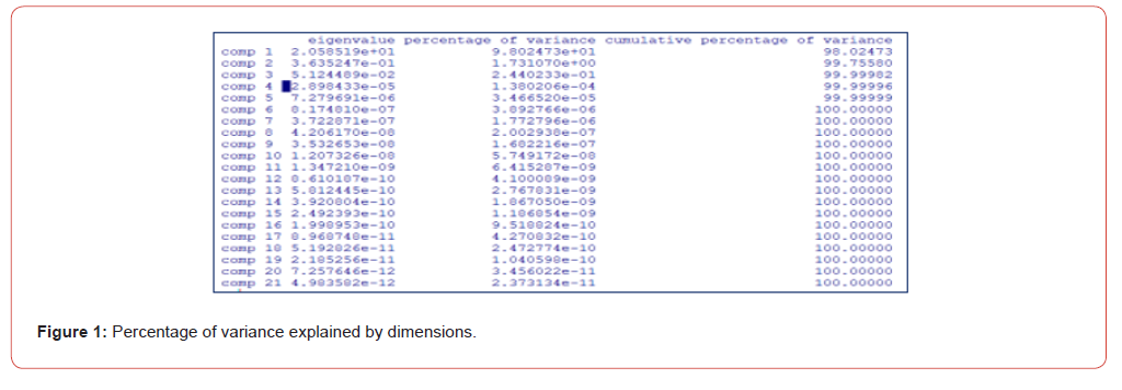
Below, we give the results of the PCA of our dataset: Note that the large variation is held by the main component 1: 98.024 % From the graph above, we might want to stop at the first main component. 98% of the information (variances) contained in the data is retained by the first main component (Figure 1).

Correlation Circle

The correlation between a variable and a Principal Component (PC) is used as the coordinates of the variable on the principal component. The representation of the variables differs from that of the observations: the observations are represented by their projections, but the variables are represented by their correlations [1] [6] (Figure 2).

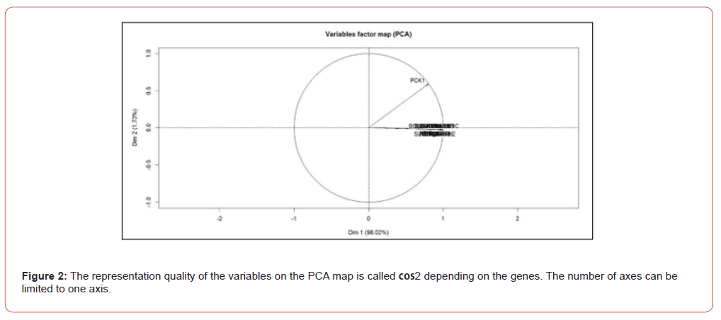
The graph above is also known as a correlation graph of variables. It shows the relationships between all the variables. It can be interpreted as follows:
• Positively correlated variables are grouped together.
• Negatively correlated variables are positioned on opposite sides of the chart origin (opposite quadrants).
• The distance between the variables and the origin measures the quality of representation of the variables.
• Variables that are far from origin are well represented by the PCA.

Note that almost all variables are correlated and contained in axis 1.
• A low 𝑐𝑜𝑠2indicates that the variable is not perfectly represented by the main axes. In this case, the variable is close to the center of the circle.

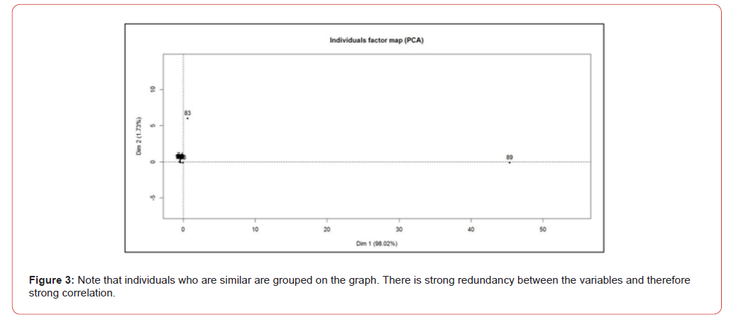
It can therefore be deduced from the obtained results that these transcriptomic data do not allow obtaining a model that discriminates in the absolute sense, despite the relatively near-acceptable performance. Consequently, these data are not exploitable. It therefore appears that these data are highly correlated indicating a single group of individuals whose variance is practically collinear with axis 1 and more or less representative since 𝑐𝑜𝑠2is less than or equal to 1 (Figure 3).

PCA was calculated using the PCA function [Factor Mine R]. Then we used the R factor extra package to produce a ggplot2 visualization of PCA results. The data is strongly correlated, and the principal component number can be reduced to a single component (axis_1). The result is the impossibility of defining a mathematical model, because all the inertia (variability) is carried by a single principal component (component_1). The complete analysis of this data stops there, no need to continue the treatment, thus saving time for the user. We can visualize the 𝑐𝑜𝑠2variables on all dimensions using the package corrplot.

It can therefore be deduced from the obtained results that these transcriptomic data do not allow obtaining a model that discriminates in the absolute sense, despite the relatively near- acceptable performance. Consequently, these data are not exploitable. It therefore appears that these data are highly correlated indicating a single group of individuals whose variance is practically collinear with axis 1 and more or less representative since 𝑐𝑜𝑠2 is less than or equal to 1.

1. S Dray (2008) On the number of principal components: a test of dimensionality based on measurements of similarity between matrices. Comput Stat Data Anal 52: 2228-2237.
2. HT Eastment, WJ Krzanowski (1982) Cross-validatory choice of the number of components from a principal component analysis. Technometrics 24: 73-77.
3. JE Jackson (1991) A User’s Guide to Principal John Wiley & Sons.
4. IT Jollife (1991) Principal Component Analysis: 2^nd Springer-Verlag, New York USA.
5. PR Peres-Neto, DA Jackson, KM Somers (2005) How many principal components? stopping rules for determining the number of non-trivial axes revisited. Comput Stat Data Anal 49(4): 974-997.
6. JV Stone (2004) Independent Component Analysis: A Tutorial Introduction.