The Quantum Equations of Numbers and Numerical Functions and Real Quantum Marker and Relation of the Degradation of Matter

The solutions of the numerical equations that I have done are more and more suitable for it to give a new aspect it is the quantum marker and the material degradation equation that demonstrates that the mass can be degraded depending energy and that the energy can be degraded according to the mass but they are complete both. the four quantum equations thus obtained are reduced to two equations two by two which will give us a new look at the quantum equations numerical functions. For the reference, it consists of two perpendicular axes that will give us a view of the quantum equations and will allow us to represent the numerical numbers according to their quantum positions.

Calculation of quantum equations of numerical numbers:

4 symmetrical quantum equations 2 to 2; So there are 2 equations in total:

First equation

We have:

The equation of numbers from 0 to N is:

This equation corresponds for the interval : [ 1^E ,1^E′ ]

Second equation

We have:

The equation of numbers from 0 to N is:

This equation corresponds for the interval: [ 1^E ,1^E′ ]

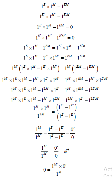
Third equation

Third equation

The equation of numbers from 0 to N is:

This equation corresponds for the interval: [ 1^E ,1^E′ ]

Third equation

We have :

The equation of numbers from 0 to N is:

This equation corresponds for the interval: [1^M ,1^M′ ]

Fourth equation

We have:

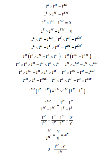
The equation of numbers from 0 to N is:

This equation corresponds for the interval: [1^M ,1^M′ ]

This guides us to make the quantum marker of numerical numbers appear as follows:

We have:

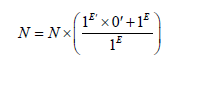
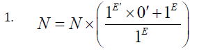
equation 1 is of the form:

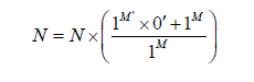
1) equation 2 is of the form:

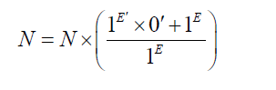
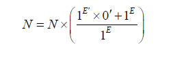
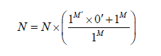
Which gives us appearance of two equations of the number N as follows:

Note:

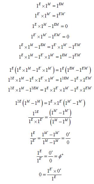
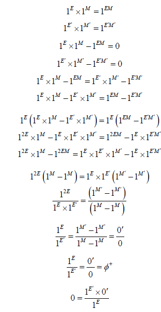
• One can make a conclusion of the previous equations to have an equation as follows:

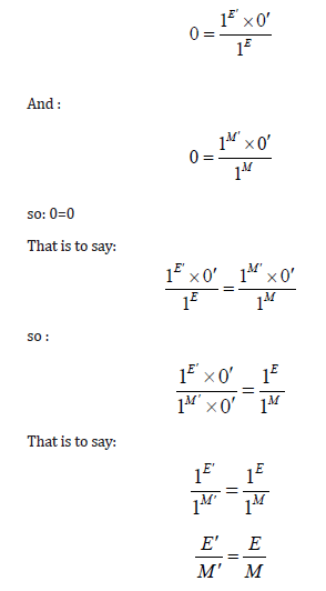
This equation is the quantum homogeneity equation. It represents the homogeneous state of matter in both cases:

The normal case (°) and the varied case (‘) this equation represents a stability between two completely different states.

If we cancel the base 1 we will have this equation which is the normal equation as follows:

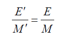
Who gives us the next new relationship:

This equation explains the degradation of matter between two different states either by energy or by mass.

Quantum landmark

The quantum marker is formed of two axes and two intervals which represent the set of the full void ∅+ and the number 0.

This representation is the best representation of quantum numbers with energy and mass.

Landmark

This is a representation of the quantum marker of numerical numbers in full empty space to the left and to the right in this representation the vertical numbers are the numbers true their image to the left and to the right represents the quantum number. We can have a multitude of representations and it remains a simple example. NB: this landmark gives us a quantum explanation of the particles in another way. When a particle has the probability of being in a place and this probability of presence of this particle is between two cases either by the existence of this particle or the nonexistence of this particle this reference is the exact translation of this state. it gives us exactly two quantum states of the particle with two different equations at the same time; I’m going to call it: the global existence.

None.

No conflict of interest.

1. Larman DG, Rogers CA (1976) Durham Symposium on the Relations between Infinite-Dimensional and Finite-Dimensional Convexity. Bulletin of the London Mathematical Society 8: 34-37.
2. Jonsson B, Nilsson M (2001) Transitive Closures of Regular Relations for Verifying Infinite-State Systems. International Conference on Tools and Algorithms for the Construction and Analysis of Systems.
3. Araki H (2004) Representations of the Canonical Commutation Relations Describing a Nonrelativistic Infinite Free Bose Gas. Journal of Mathematical Physics 4: 637.
4. Jonsson B, Nilsson M (2001) Transitive Closures of Regular Relations for Verifying Infinite-State Systems. International Conference on Tools and Algorithms for the Construction and Analysis of Systems.
5. Araki H (2004) Representations of the Canonical Commutation Relations Describing a Nonrelativistic Infinite Free Bose Gas. Journal of Mathematical Physics 4: 637.