


 Research Article
Modelling Colinearity in the Presence of Non–Normal Error: A Robust Regression Approach
Received Date: July 15, 2019 Published Date: July 26, 2019
Abstract
Multicollinearity and non-normal errors, which lead to unwanted effect on the least square estimator, are common problems in multiple regression models. It would therefore seem important to combine estimation techniques for addressing these problems. In the presence of multicollinearity and non-normal errors, different estimation techniques were examined, namely, the Ordinary Least Squares (OLS), Ridge Regression (R), Weighted Ridge regression (WR), Robust M-estimation (M), and Robust Ridge Regression with emphasis on M-estimation (RM). When compared with the condition of Collinearity, the results of a simulated study shows that Robust Ridge (RM) provides a more efficient estimate then the other estimators considered. When both Collinearity and non-normal errors were considered, the M-estimators (M) produces a more efficient and precise estimates.
Keywords: Multicollinearity; Ordinary least squares (OLS); Regressor; Simulation; M-estimator; Estimates
Introduction
Regression analysis is “robust” in that it will typically provide estimates that are reasonably unbiased and efficient even when one or more of the assumptions is not completely met. However, a large violation of one or more assumptions will result in poor estimates and, consequently, the wrong conclusions being drawn. Two important problems are considered in regression analysis: multicollinearity and non–normal error distribution. Multicollinearity is the term used to describe cases in which the regressors are correlated among themselves. Another common problem in regression estimation methods is that of non–normal errors. The term simply means that the error distributions have fatter tails than the normal distribution. These fat–tailed distributions are more prone than the normal distribution to produce outliers, or extreme observations in the data. The Ordinary Least Squares estimators (LS) of coefficients are known to possess certain optimal properties when explanatory variables are not correlated among themselves, and the disturbances of the regression equation are independently, identically distributed normal random variables. This study focuses on violation of the assumption that there is no linear relationship between the explanatory variables and the disturbances distribution is non–normal. If this assumption is violated, multicollinearity ensues which leads to inflation of Standard Error (SE) of the coefficients of the estimated parameters [1-6]. Multicollinearity is a case of multiple regression in which the predictor variables are themselves highly correlated, meaning that one can be linearly predicted from the others with a non–trivial degree of accuracy. If there is no linear relationship between the regressors, they are said to be orthogonal. When the regressors are orthogonal, the inferences such as;
(i) identifying the relative effects of the regressor variables,
(ii) prediction and/or estimation, and
(iii) selection of an appropriate set of variables for the model
Can be made easily. Unfortunately, in most applications of regression, the regressors are not orthogonal. Sometimes the lack of orthogonality is not serious. However, in some situations the regressors are nearly perfectly linearly related, and in such case the inferences based on the regression model can be misleading or erroneous. When there are near–linear dependencies among the regressors, the problem of multicollinearity is said to exist. Non–normal error is a situation whereby the errors have fatter tails than the normal distribution tail. The Gauss-Markov Theorem says that OLS estimates for coefficients are BLUE when the errors are normal and homoscedastic. When errors are nonnormal, the ‘E’ property (Efficient) no longer holds for the estimators and in small samples, and the standard errors will be biased. When errors are heteroscedastic, the standard errors become biased. Thus, we typically examine the distribution of the errors to determine whether they are normal.
M – Estimation
The theory of robustness developed by Huber and Hampel (1960) laid the foundation for finding practical solutions too many problems, when statistical concepts were vague to serve the purpose. Robust regression analyses have been developed as an improvement to least squares estimation in the presence of outliers and to provide us information about what a valid observation is and whether this should be thrown. The primary purpose of robust regression analysis is to fit a model which represents the information in the majority of the data. Robust regression is an important tool for analyzing data that are contaminated with outliers. It can be used to detect outliers and to provide resistant results in the presence of outliers. Many methods have been developed for these problems. Many researchers have worked in this field and described the methods of robust estimators. The class of robust estimators includes M-, L- and R-estimators. The M-estimators are most flexible ones, and they generalize straightforwardly to multiparameter problems, even though they are not automatically scale invariant and have to be supplemented for practical applications by an auxiliary estimate of scale any estimate [6-10].
Motivation
This research work was motivated by the idea that in the presence of substantial collinearity and non–normal error in a regression model, the results obtained from Ordinary Least Square Estimator are unreliable. The effect and remedy to such influences needs to be study.
Material and Methods
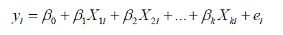
The basic requirement of the LS estimation of a linear regression
is that  exits. The two major reasons that the inverse does not exit is (1) when > n , (2) multicollinearity. When multicollinearity
exits the design matrix is “ill conditioned” and invertible. A simple
way to guarantee the invertibility is adding a constant to the
diagonal matrix
exits. The two major reasons that the inverse does not exit is (1) when > n , (2) multicollinearity. When multicollinearity
exits the design matrix is “ill conditioned” and invertible. A simple
way to guarantee the invertibility is adding a constant to the
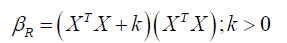
diagonal matrix  before estimating the coefficients. Hoerl
and Kennard (1970) proposed the ridge estimator
before estimating the coefficients. Hoerl
and Kennard (1970) proposed the ridge estimator
Another way of understanding the ridge estimator is; recall that
the LS estimator2 tends to minimizes the residual sum square i.e.
 but when
collinearity exist then ˆβ
is sensitive to small change in the data
set and we uses ridge estimator that penalizes the value of β by
minimizing
but when
collinearity exist then ˆβ
is sensitive to small change in the data
set and we uses ridge estimator that penalizes the value of β by
minimizing
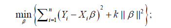
The first term of equation (3.1.5) is regarded as the loss and the second term of the equation is the penalty. Note that: with larger k the penalty of β becomes stronger [10-14].
Robust regression methods
Robust Regression estimators have been proven to be more reliable and efficient than Least Squares Estimator especially when disturbances are non-normal. “Non-normal disturbances” are disturbances distribution that have heavy and fatter tails than the normal distribution and are prone to produce outliers. Since outliers greatly influence the estimated coefficients, standard errors and test statistics, the usual statistical procedure may be most inefficient as the precision of the estimator has been affected. Several different classifications of robust regression exist. Two of the most commonly considered group are: L-estimators and M-estimators. The L-estimators is the earliest one. One important member of regression L-estimators is called Weighted Least Squares estimator (WLS).
Weighted Least Squares Estimator
Given a regression model: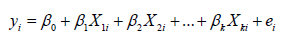 where are random errors that is independent and identically distributed with mean zero and variance . Suppose we have
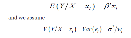
where 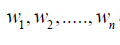 are known positive numbers.
The model can now be re-written as
are known positive numbers.
The model can now be re-written as
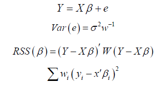
The Weighted Least Squares estimator also known as the Generalized Least Squares estimator is given by:
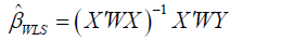
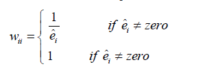
where W is a diagonal matrix with diagonal elements. The diagonal elements of W matrix are set equal to:
M - Estimation
The linear model:
This can also be written in matrix form as:
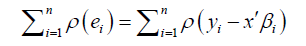
The general M-estimator minimizes the objective function
Robust ridge regression estimates
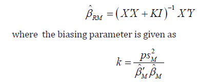
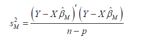
The following formula is used to compute robust ridge estimates:

where  denotes the coefficient estimates from the robust estimators. Many methods of selecting appropriate k values have
been proposed in the literature. In this study, the method proposed
by Hoerl, Kennard and Baldwin (HKB) (1975), based on Least
Squares estimator, has been used for the selection of the k values,
building on robust estimators:
denotes the coefficient estimates from the robust estimators. Many methods of selecting appropriate k values have
been proposed in the literature. In this study, the method proposed
by Hoerl, Kennard and Baldwin (HKB) (1975), based on Least
Squares estimator, has been used for the selection of the k values,
building on robust estimators:
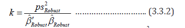
where p is the number of regressors and  is the robust
scale estimator.
is the robust
scale estimator.
Weighted ridge estimator (Wr)
Weighted Ridge Estimator  can be computed using the
following formula:
can be computed using the
following formula:
βW denotes the coefficient estimates from the Weighted Least
Square estimators. The Ridge M-estimator of the parameter β is given by: where the M-estimator procedure of is used rather than Least
Square estimator in computing and values in order to reduce the
effect of non-normality on the value choosen for , and the value can
be written as: [16-18]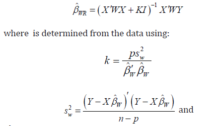
Ridge M-Estimator (Rm)
Results and Discussion
Data simulation
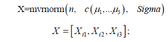
The data utilized for this work were simulated from R (www. cran.r-project.org) statistical package. The three predictor variables are generated form the multivariate normal package as follows:
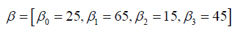 is the vector of the
true population value that the data set is simulated from.
is the vector of the
true population value that the data set is simulated from.
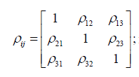 the specified correlation and it varies
between Tolerable Non-Orthogonal Correlation Point and the
extreme correlation
the specified correlation and it varies
between Tolerable Non-Orthogonal Correlation Point and the
extreme correlation
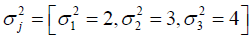 is the variance vector of the
predictors.
is the variance vector of the
predictors.
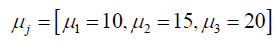 is the specified mean vector
of the predictors.
is the specified mean vector
of the predictors.
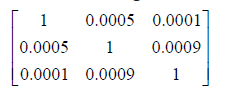
Sigma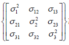 Variance cov ariance matrix
One important factor in this study is the disturbances distribution. Therefore, the residual term was simulated from two distributions, namely:
• The univariate normal distribution with mean 0 and standard deviation σ =10, and
• Cauchy distribution with median zero and scale parameter one
e1 = rnorm(n ∗ p,0,σ )
e2 = rcauchy (n ∗ (1− p),0,1)
e = c (e1,e2)
Where p represents the proportion of error from the normal distribution.
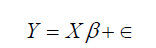
Y = Xβ +ε
And the response is simulated with the relationship given below
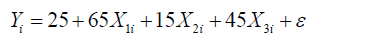
is the vector of the generated dependent
variable.
Correlation structure
For the TNCP (tolerable non orthogonal correlation)
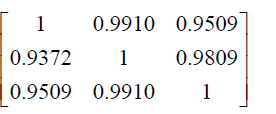
For the severe correlation
In order to compare the performance of the estimators, the Mean Square Error (MSE) was computed for the data set at various sample sizes and at different iteration. In each case, the average MSEs for each sample were reported. The true parameter values were compared with the regression estimates at different sample sizes (Table 1).
Table 1: Summary of Estimate of Coefficients and Standard Error at Various Sample Size for Tolerable Non-Orthogonal Correlation.
From Table 1 it is observed that the value of estimated regression coefficients for all the estimators considered is an unbiased estimate of the population parameter when the regressors are orthogonal, and the disturbances of the regression equation are independent, identically distributed normal random variables, except for Weighted Ridge which is over estimating the parameter (Table 2).
Table 2: Mean Square Error of the estimators at various sample sizes.
From Table 2, it is observed that the MSEs asymptotically tend to zero as the sample sizes become large, which is indicating the consistency of the estimators except that of the Weighted Ridge which is not stable (Table 3).
Table 3: Summary of Estimate of Coefficients and Standard Error At Various Sample Size for Severe Correlation Level.
From Table 3, it is observed that the result obtained from Weighted Ridge is inconsistent with true parameter and result obtained from other estimators considered in this study. It is also observed that as the sample sizes become large, the result obtained from other estimators except Weighted Ridge converges to the true parameter (Table 4).
Table 4: Mean Square Error of the estimators at various sample sizes.
From Table 4, it is observed that the MSEs asymptotically tend to zero as the sample sizes become large, which is indicating the consistency of the estimators except that of the Weighted Ridge which is not stable. Where the MSE of Robust Ridge clearly show that it is more efficient than other estimator considered (Figure 1).
From the plot above, it is observed that the MSE asymptotically tend to zero as the sample sizes becomes large, which indicate the consistency of the estimators (Table 5).
Table 5: Summary of Estimate of Coefficients and Standard Error At Various Sample Size for Tolerable Non-Orthogonal Correlation.
From the above table, it is observed that the result obtained from Robust M-estimation is an unbiased estimate of the true parameter, while result obtained from other estimators considered in this study are biased which is as a result of non-normal error (Table 6).
Table 6: Mean Square Error of the estimators at various sample sizes.
From the Table above, it is observed that the MSE of M-estimation asymptotically tend to zero as the sample sizes become large, which is indicating the consistency of the estimator compared to other estimators considered in this study, while the result of MSE based on OLS is the worst among the estimators. Robust M-estimator is more efficient than other estimator considered (Table 7).
Table 7: Summary of Estimate of Coefficients and Standard Error at Various Sample Size for Severe Correlation Level.
From the above table, it is observed that the result obtained from Robust M-estimation is an unbiased estimate of the true parameter, while result obtained from other estimators considered in this study are biased which is as a result of effect of collinearity and non-normal error (Table 8).
Table 8: Mean Square Error of the estimators at various sample sizes.
From the table above, it is observed that the MSE of M-estimation asymptotically tend to zero as the sample sizes become large, which is indicating the consistency of the estimator compared to other estimators considered in this study, while the result of MSE based on OLS is the worst among the estimators. Robust M-estimator is more efficient than other estimator considered (Figure 2).
Conclusion
From the simulation studies it can be concluded to a reasonable extend that In the presence of both multicollinearity and nonnormal error the OLS estimators produces relatively large Mean Squares Errors, hence it gives unstable parameter estimates. the sample size is inversely proportional to the mean square error of estimate i.e. the larger the sample size, the lower the mean square error and vice versa. To make any reasonable predictions and inferences in any multiple linear regressions, one must be certain that the predictors are non-orthogonal and the percentages of data that are outliers are minima before the commencement of the analysis. This study reveal that the consequence of collinearity in the presence of non-normal error is more severe compared to when the error distribution is normal. Finally, the results of comparisons shows that for the condition of collinearity, Robust Ridge estimates are more efficient than the other estimators considered. While for the condition of collinearity and non-normal error M-estimator produces estimates that were more efficient and precise.
Recommendation
This research work will help present and future researchers in choosing or determining the appropriate estimator for estimating the regression parameters when the traditional method for estimating the parameters is unreliable in the presence of both multicollinearity and non–normal error problem in a data set.
Acknowledgement
None.
Conflict of Interest
No conflict of interest
References
- Askin GR, Montgomery DC (1980) Augmented robust estimators. Technometrics 22(3): 333-341.
- Belsley DA, Kuh E, Welsch RE (1980) Regression Diagnostics: Identifying influential Data and Sources of Collinearity. John Wiley & Sons, New York.
- Babalola AM, Obubu M, Otekunrin OA, Obiora-Ilono H (2018) Selection and Validation of Comparative Study of Normality Test. American Journal of Mathematics and Statistics 8(6): 190-201.
- Babalola AM, Obubu M, George OA, Ikediuwa CU (2018) Reprospective Analysis of Some Factors Responsible for Infant Mortality in Nigeria: Evidence from Nigeria Demographic and Health Survy (NDHS). American Journal of Mathematics and Statistics 8(6): 184-189.
- Moawad El-Fallah Abd El-Salam (2013) The Efficiency of some Robust Ridge Regression for Handling Multicollinearity and Non-normals Errors Problems. Applied Mathematical Sciences 7(77): 3831-3846.
- Farrar, Glauber (1967) Multicollinearity in Regression Analysis. Review of Economics and Statistics 49: pp. 92-107
- Gujarati DN (2004) Basic Econometric 4th edition. Tata McGraw-Hill, New Delhi, India.
- Hoerl AE, Kennard RW (1970) Ridge regression: Biased estimation for non-orthogonal problems. Technometrics 12: pp. 55-67.
- Hoerl AE, Kennard RW (1970) Ridge regression: Applications to non-orthogonal problems. Technometrics 12: pp. 69-82.
- Hoerl AE, Kennard RW, Baldwin KF (1975) Ridge regression: Some simulations. Communications in Statistical Theory 4(2): 105-123.
- Holland PW (1973) Weighted ridge regression: Combining ridge and robust regression methods. NBER Working Paper 11: 1-19.
- Huber PJ (1964) Robust estimation of a location parameter. Annals of Mathematical Statistics 35(1): 73-101.
- Montgomery DC, eck EA (1982) Introduction to Linear Regression Analysis. Wiley, New York, USA.
- Rawlings JO, Pantula SG, Dickey DA Applied Regression Analysis. A Research Tool.
- Samkar Hatice, Alpu Ozlem (2010) Ridge Regression Based on Some Robust Estimators. Journal of Modern Applied Statistical Methods 9(2): 17.
- Silvapulla MJ (1991) Robust ridge regression based on an M-estimator. Australian Journal of Statistics 33(3): 319-333.
- Obubu M, Babalola AM, Ikediuwa CU, Amadi PE (2019) Parametric Survival Modeling of Maternal Obstetric Risk; a Censored Study. American Journal of Mathematics and Statistics 9(1): 17-22.
- Obubu M, Babalola AM, Ikediuwa CU, Amadi PE (2018) Modelling Count Data; A Generalized Linear Model Framework. American Journal of Mathematics and Statistics 8(6): 179-183.
-

This work is licensed under a Creative Commons Attribution-NonCommercial 4.0 International License.


