Chance or Causality in Human Genetics?

Deciding whether events are due to causal effects or only arise by chance is one of the most important judgements to make in the research laboratory (and possibly in daily life as well). In genetics random events are supposed to occur at the separation of alleles into germ cells at meiosis and at fusion of germ cells during fertilization; and causal events occur with diseases arising from a point mutation such as cystic fibrosis or sickle cell anemia. Is there a real difference in the results of paired replicate experiments compared with controls or is it just due to random events or chance? Random events may of course only seem so due to incomplete information about the process under study.

Getting the choice right between chance or causal events in the research laboratory can be as important as doing the experiments; years and money can be wasted with a project that comes to nothing if one makes the wrong probability decisions from the start. Methods are provided by statisticians to assign numbers to probability values for the differences between means and variances of samples to decide whether the experimental data is significantly different from the control data or not [1]. A probability test to decide whether an injection of insulin will lower the blood sugar is probably not required; it does so almost every time since one is so close to the central biochemistry of the reaction. But many other causal effects in medicine and genetics are statistical in nature, occurring as group averages and not necessarily observed for every individual patient or experiment; so, probability tests have evolved. Even in such an exact science as physics similar conditions are found. For example, Boyles Laws states there is an inverse relationship between pressure and volume of a gas in a container. The pressure depends on the number of molecules of gas impinging on the wall of the vessel and over some square millimeters of the wall there may be no molecules colliding; whereas over another square millimeter there may be many. So the pressure in the container is a statistical average of the number of molecules hitting the wall over a particular time interval; and it is surprising that it can be expressed in such simple algebra as pressure (p)=K₁/volume (v), where K is a constant depending on the nature of the gas.

The problem for genetics is the simplest of books on statistics describe more than 17 probability tests (zM, Yates, Student’s t, Wilcoxon, Kruskal Wallis, Friedman, Fisher, Cochran etc.) to calculate the probability as to the experimental sample being truly different from the control population [2]. They come with all sorts of conditions and limitations of when and how to use them. One colleague plugged his data through them all in turn to choose a test that gave the best p value to report his data; a dangerous expedient that might only result in fooling himself.

The formulae for these tests often appear excessively complicated perhaps appealing to the mind of a mathematician but not necessarily to a biologist or geneticist. For example, the Student’s t test is commonly used for small samples, but the data are required to be independent measurements and their distribution to fit a Gaussian or normal curve. The formula for the single-tailed Student’s t distribution is [3]:

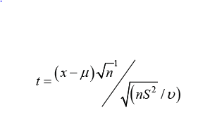
Where x = mean of controls μ = mean of sample, n= number of comparisons, S = Standard Deviation, and v = degrees of freedom.

The difference of the means is straight forward but understanding the need for square of S and square root terms of n seems to require a course in basic statistics. This test depends on the probability density function of the standard normal curve (or Gaussian curve) that is:

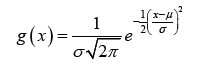
This function is even more confusing. Asking a statistician why the square root of 2 pi comes into the equation produces no good answer except that it provides the best solution to the differential equation of making the area under the bell-shaped curve equal to one; this is to satisfy one of the basic laws of probability. So why subject the results of several years’ experimental work to a formula that you do not fully understand?

Even more complicated is the following equation commonly used to calculate Fisher’s z statistic based on the distribution of variance ratios:

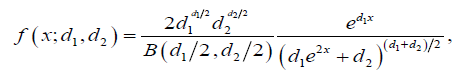
See Weatherburn [3] for assignment of coefficients and terms. This is clearly the product of a sophisticated mathematical mind and perhaps designed to bamboozle the poor geneticist. Rather than having a dogmatic faith in these incomprehensible tests it would be nice to have a probability test that is completely comprehensible, can be calculated with pen and paper without having to use extensive tables or computers, and preferably can be done by mental arithmetic.

Such a test exists for comparing paired replicates and is based on the binomial distribution of discrete random variables using the function of ‘greater than’ or ‘less than’ (< x or x <). To simplify the ideas behind the test, if a coin is tossed 6 times and it comes down tails each time it is correct to claim this would be due to chance with a probability of 1/64 = 0.014, so therefore the coin may be biased in some way. If it came down tails 30 consecutive times, then it would certainly be biased. Both would be counted as a significant result for many genetic experiments i.e. signifying a less than 5% chance of the results being due to random events. One simple equation to calculate this is:

Equation 1. P = 1/2N. N! /r! (N-r)!

Where P is the probability value, N is the number of experiments done and r is the number of successful outcomes according to the hypothesis to be tested [4].

This formula is based on combinations as used in the binomial theorem and represents the ratio of all possible outcomes of the controls to all possible outcomes of the experiments where the order taken is unimportant. Thus if the ranked experimental results come out less (or more than) the control measurements in a timeordered sequence and let this be called ‘tails’; then if repetition of six experiments produces 6 ‘tails’ then the p-value of the results as being due to random effects is 1/64 = 0.014.

Professional statisticians in the UK can be dismissive of this binomial (or non-parametric) test: it is too simple, it is not very powerful, one needs at least 5 paired comparisons in the same direction to make it work (1/32 = 0.031) etc. In its favor it does not make any assumptions about a Gaussian or any other distribution of the data and its comprehensibility trumps many of the disadvantages.

It is designed to evaluate the significance of differences of discrete random variables compared to controls but can be easily used to test the significance of continuous random variables by converting the results into a function such as ‘more than (>) or less than (<)’, of the numbers of comparisons made between experimental and controls samples in a time-ordered or any other sequence not based on magnitude.

On further discussions statisticians even with such a simple equation, irrationality intrudes. If as in the previous example the number of experiments N equals the number of successes (r) the term (N-r)! appears in the denominator i.e. 0! which in one sense should be equal to zero ( numbers multiplied by zero are zero ) and the whole formula falls to pieces becoming 0. But not according to mathematicians; 0! =1. Enquire again for an explanation of this and there appears to be no convincing answer [5].

One answer is by completing the following notation of factorials: 3! =4! /4 =6; 2! = 3! /3 = 2; 1! =2! /2 = 1; leading to 0! = 1! /1 = 1. However, if one considers the next step of factorial -1 one gets 0! /0 = 1/0 = ∞ (infinity) which becomes nonsense; in the number system -1! cannot equal ∞. Another ‘proof’ that 0! =1 comes from set theory and permutations. Thus, the permutations of 3 objects taken three at a time in a set is 3! = 6; two objects taken 2 at a time is 2! = 2, with 1 object it is 1! = 1; therefore, continuing the pattern taking 0 objects 0 at a time is 0! = 1; thus, meaning an empty set can only be ordered in one way.

Inconsistencies occur in both answers and it might be more straightforward to state 0! = 1 is a convention, purely to make some equations like Equation 1 work better even though any proof is incomplete. In other situations 0× 0× 0 recurring = 0; so neither can be counted as axioms.

Kurt Godel (1906-76), an Austrian logician and mathematician, derived two incompleteness theorems related to this topic which showed [6]: 1. That in any axiomatic system, such as arithmetic, there are propositions of a comparatively elementary nature that could be true but cannot be deduced from within the system; and 2. He also concluded that a definitive proof of consistency within the system must be given up altogether. An elementary account of his theorems is treated in Chapter 4 of Fundamental Concepts of Mathematics [7].

It is disquieting to find such uncertainty appearing so early in such a simple numerical test for assigning probability values that research laboratories have used for years. It makes one wonder how many other inconsistent propositions are contained in the more complicated probability tests that we overlook due to incomprehension. These tests should perhaps be taken just as pointers to which investigations are worthy of further study and not as a proof of the truth of the proposition. Perhaps the only solution is to learn to do and understand them whatever contradictions they may contain. Independent replication of experiments, especially by alternative methods and in different laboratories, may be a much better guide to the truth or importance of a proposition than these mathematically assigned numbers for probability. The gold standard for proof of the truth or otherwise of experimental work must still remain its ability to predict the future outcomes of the phenomena under study.

The author wishes to thank Professor John Walker- Smith and Professor Kenneth Harris for helpful comments.

No conflict of interest.

1. Backhouse J K (1971) Mathematical topics: an introduction to tests of significance. Longman Group, London, UK.
2. Langley R (1970) Practical Statistics. Pan Books Ltd. London, UK.
3. Weatherburn CE (1968) A First course in Mathematical Statistics. Cambridge University Press, UK.
4. Siegel S (1956) Non-parametric Statistics. McGraw-Hill, New York, USA.
5. Weyl H (1947) Philosophy of Mathematics and Natural Science. Princeton University Press, USA.
6. Godel K (1931) Uber formal Unentscheidbare Satze der Principia Mathematica. Math Phys 38: 173-198.
7. Goodstein RL (1962) Fundamental Concepts of Mathematics. Pure and Applied Mathematics, Pergamon Press Ltd, Oxford, UK, p. 22.