Semi-Parametric Bayesian Estimation of Sparse Multinomial Probabilities with An Application to The Modelling of Bowling Performance in T20I Cricket

Introduction

Categorical data are often analyzed using multinomial data, and sparseness in multinomial data is frequently encountered in practice when many cells have small and/or zero counts. Such sparse multinomial data can arise in two ways (1). relatively few observations are dispersed in numerous categories, or (2). cells that are structurally empty, i.e., theoretically impossible to observe. Assume, for instance, that K cells have probabilities p₁, p₂, ..., p_K of occurring. Then, under the first scenario, many cells have a small probability pi relative to the number of observed outcomes leading to small or even zero counts. In this case, increasing the number of effective observations by combining different data sources could help to improve inference. It is the approach we take here. Under the second scenario, however, some cells have a probability pi = 0 of occurrence. Identifying those structural zeros becomes a central part of the inference problem.

In this manuscript, we focus on the case of sparse multinomial data that are due to the observations dispersed in numerous categories or when the number of observations is small relative to the number of categories. The Maximum Likelihood Estimator (MLE) performs very poorly in this setting. Shrinkage estimation is an approach that allows for deriving improved estimators, and in particular, it can handle certain forms of sparsity by borrowing information from other multinomial populations. Our main objective is to develop an improved strategy to jointly estimate the cell probabilities of m multinomial populations in the context of sparse data.

The paper will proceed as follows. In Section 2, we discuss the previously studied statistical models, including James-Stein (JS) estimation, empirical Bayes (EB) estimation, and estimation based on Bayesian multinomial regression. In Section 3, we discuss the proposed statistical model, semi-parametric Bayesian estimation. In Section 4, we apply the methods presented in Sections 2 and 3 to data consisting of the bowling performance of 175 players over ten years. We also conducted a simulation study to compare the methods. We conclude with a short discussion in Section 5 based on the results and methods presented in the paper.

Standard Statistical Models and Estimation

In summarizing the bowling performance of a player in cricket, the total number of wickets taken by a bowler can be divided into K discrete categories (more details will be provided in Section 4). Specifically, assume we have m bowlers and let n_i be the total number of matches the i^th bowler has played, and X_ij be the number of matches in which the i^th bowler has taken exactly j−1 wickets, j = 1, ..., K. We can naturally model these categorical outcomes using the multinomial distribution as follows;

given by

for i = 1, 2, ..., m. Note that the cell counts in some categories will be either small or zero, which will result in a sparse table. In this case, the Maximum Likelihood Estimator (MLE) of p_ij, denoted by, p_ij^MLE performs very poorly and underestimates the true cell probabilities (pij) due to sparsity. To help to mitigate this problem, the James-Stein approach can be used to estimate pij.

James-Stein estimation

The concept of shrinkage was first introduced in statistics by [1], and the general principles behind shrinkage estimation were discussed by [2]. The famous James-Stein shrinkage estimator was introduced by [3], which is based on a weighted average of two different models; a high-dimensional model with low bias and high variance and a lower-dimensional model with larger bias but smaller variance.

Suppose that the shrinkage target T is associated with the lower- dimensional model with smaller variance and considerable bias and that U is associated with the high-dimensional model with low bias and high variance. In shrinking, we try to find a compromise between T and U by computing a convex linear combination,

instead of choosing between one of the models. U * is called a shrinkage estimator, and it often outperforms the individual estimators T and U in terms of accuracy and statistical efficiency [4].

Here λ is usually a number between 0 and 1 and is called the shrinkage constant. It measures the weight that is given to the shrinkage target T. If λ = 1, the shrinkage estimate equals the shrinkage target T, whereas, for λ = 0, it equals U. This strategy has been used to estimate the cell probabilities of a multinomial distribution;

where t_j is the shrinkage target. Note that p_ijJS is improved over MLE by combining the player-specific information given by the MLE with a target t_j that provides “global” information relevant to all populations. The default choice of k_j = 1/k is convenient but less than optimal in most cases. A popular shrinkage target (t_j) is the overall proportion of observations in category j. It seems appropriate to choose the population-specific shrinkage constant λ_i in a data-driven fashion by minimizing the mean squared error (MSE) of the resulting estimator. Assuming that the first two moments of the distributions of t_j exist, it can be shown that

Then, the optimal shrinkage constant *λ_i can be obtained by analytically minimizing this function with respect to λ_i, leading to

Given that p_ijMLE is an unbiased estimator for p_ij and following Ledoit and Wolf (2003), we can further simplify the above expression to

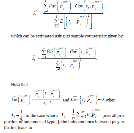
Empirical Bayes estimation

One can also take an empirical Bayes approach for estimating pij by following the development in [5]. First, assume that each pi has the same prior distribution;

Then, the posterior distribution of pi, given the observed counts for player i, is

which is a shrinkage estimator with

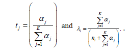
Here t_j is the shrinkage target corresponding to the prior mean of p_ij and (0,1) i λ ∈ is the shrinkage constant. Then, the empirical Bayes strategy is to replace the shrinkage target and constant with their sample counterparts,

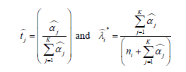
in the above expression for the Bayes estimator. The parameter estimates α = (α₁,α₂ αK)^t are obtained by using the dirmult package in R [6], relying on maximum likelihood estimation based on the marginal distribution of the data given α, and can be interpreted as using data-driven parameters in the prior distribution.

Bayesian multinomial regression estimation

We now describe a Bayesian multinomial regression approach for estimating p_ij in the presence of covariates. Let Y = (Y₁, Y₂, ..., Y_l) represent an m×l matrix of l covariates for the m players, where Y_l = (Y_1l, Y_2l, ..., Y_ml)t. In the Bayesian multinomial regression model formulation, we write our estimation problem as

Here α_i is positive, and a natural link function is a log-link function leading to

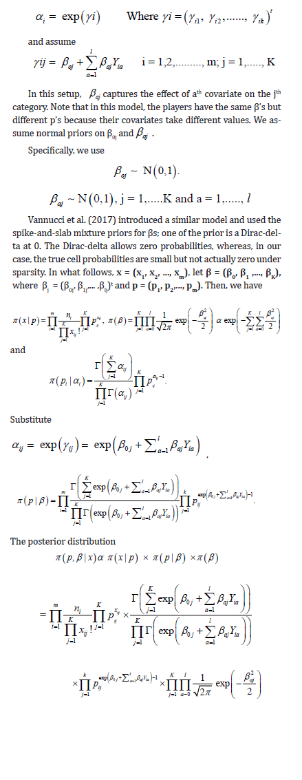
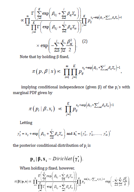
So that the posterior conditional distribution of β (given p) does not belong to a standard family of distributions. To perform inference based on the full posterior distribution (2), we developed a Metropolis within Gibbs algorithm to generate values from this distribution. Alternatively, Bayesian multinomial logistic regression could have been used in the current context. In multinomial logistic regression, we nominate one of the categories to be a baseline or reference category (usually the last category), calculate log odds for all other categories relative to the baseline, and let the log odds be a linear function of the predictors as follows:

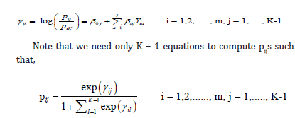
Note that we need only K − 1 equations to compute pijs such that,

In the Bayesian setting, we put priors on β_0js and β_ajs. One important advantage of our proposed multinomial regression model is that it derives a distribution for pi instead of calculating p_ij’ separately as the multinomial logistic regression model.

Proposed Semi-parametric Bayesian Estimation

Our focus is mainly on data sparsity, which means cell counts are small for one or more categories due to the small sample size and the cell probabilities are small but not actually zero. However, the conventional multinomial models perform very poorly under sparsity. We aim to develop an approach to derive improved estimators that can handle sparsity by borrowing information from other multinomial populations. The Dirichlet process is one of the most popular Bayesian non-parametric models. The primary motivation to use the Dirichlet process as a prior distribution is that it gives a large space over which we make our inferences as well as a tractable posterior distribution [Teh (2010)]. Another advantage of the Dirichlet process is the clustering property which clusters the populations without specifying the number of clusters in advance. This clustering property borrows information from similar populations, which helps to handle data sparsity. With those advantages, we propose a semi-parametric Bayesian estimator based on the Dirichlet process (DP).

Dirichlet processes, introduced by [9], are a family of stochastic processes whose realizations are probability distributions. These can be seen as a distribution over distributions as each draw from a Dirichlet process is itself a distribution. It is called a Dirichlet process because it is a generalization of the Dirichlet distribution to an infinite number of dimensions to model the weights of these components. A Dirichlet process is completely specified by two components; an underlying base distribution (G₀) and a positive real number (α₀) called the concentration parameter and is denoted by

If the base distribution is continuous, then G is a discrete distribution made up of a countably infinite number of point masses. The concentration parameter α₀ is also called the strength parameter as it specifies how “strong” this discretization actually is. It can be shown that

For any measurable subset A ⊂ Θ. When α₀ →0 , all the realizations are concentrated at a single value, while in the limit of α₀ → ∞ , the realizations become continuous. We formulate our semi-parametric Bayesian model as follows;

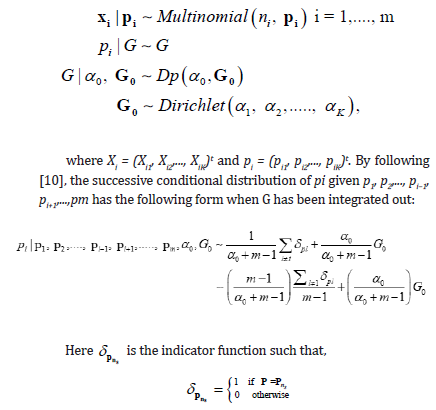
The posterior base distribution is a weighted average between the prior base distribution G0 and the empirical distribution

. The weights are controlled by the concentration parameter α0. The larger the α0 value, the larger the weight for G0 in comparison to the weight for the empirical distribution and vice versa. For m >> α0, the empirical distribution will dominate. For m → ∞, the posterior of the DP converges to the true underlying distribution over p. We refer readers to [11] for other properties of DP formulation and its properties. Note that one can use the stick-breaking construction proposed by [12] to draw samples from a DP. In the stick-breaking construction, we draw

Intuitively, consider starting with a stick of unit length and breaking a random proportion ξ1 of that stick. The length of this piece gives you the

first weight π1. Then, break a random portion from the remaining stick ξ₂. The length of the second piece gives you the second weight π₂. Now, continue breaking the remaining portions of the stick to obtain π₃, π₄, and so forth. Using this construction, an infinite sequence of weights can be generated. When ns gets larger and larger, the lengths of the pieces of the stick, or the weights, will tend to get smaller and smaller. The lengths of the pieces are determined by the concentration parameter α₀. For small α₀, only the first few pieces will have significant lengths, the remaining pieces having very small lengths. On the other hand, for large α₀, the lengths will tend to be more uniform. Then, the discrete random probability distribution is and we sample from the posterior distribution of p using the Gibbs sampling approach described in [13].

Data Analysis

Application to Inference on Bowling Performance

Some background information: The game of cricket was first started in the late 16^th century and has become popular globally in the 19^th and 20^th centuries due to the introduction of various formats, including Twenty20 international cricket (T20I cricket). Cricket has multiple formats depending on the desired length of a typical match. Test cricket has a duration of five days, and one-day cricket has a period of one day, whereas T20I matches are completed in roughly three hours, with each inning lasting about 75-90 minutes. The International Cricket Council (ICC) governs the body of cricket, with 105 countries as its members. [14-16] provides a comprehensive discussion on various aspects of cricket and its recent research directions.

There has been growing interest in T20I cricket performance analysis in recent literature. [17] provided a comprehensive overview of tactics in T20 international cricket. A simulator for modeling T20I cricket was proposed by [18]. Note that there are three major components that lead to success in cricket: batting, bowling, and fielding. [19-22] assessed the batting performance of players in the Indian Premier League (IPL) and one-day international cricket. [19] proposed a Bayesian hidden Markov model, and [22] proposed a performance measure combining batting average, batsman’s consistency, and strike rate. However, we remark that there has been little attention on bowling or fielding performance. [23] proposed an approach based on random forests to measure the fielding performance in T20I cricket. In what follows, we study the bowling performance of players in T20I cricket using the models introduced in Section 3.

About Bowling Performance in T20I Cricket: Here, we consider the number of wickets taken in T20 international matches by bowlers between 1st of January 2010 and 11th of March 2020. Our analysis includes m = 175 bowlers with at least 16 total wickets. Details of these T20I matches can be found in the Archive section of the ESPNcricinfo website (www.espncricinfo.com), and the T20I bowler rankings were obtained from the ICC cricket website (www. icc-cricket.com) on March 11, 2020. The number of matches ranged from 8 to 77 matches for each bowler. Rashid Khan is the highest wicket-taker with 89 total wickets for the given period, and he was the highest-ranked bowler on March 11, 2020, according to ICC. Recall that the basic assumption here is that

Table 1 provides the number of players (out of 175) who have non-zero counts for each wicket category. The highest number of wickets recorded in a single match by one bowler in T20 international matches was 6 wickets over the considered time period. It is clear that 6 wickets are very rarely achieved, and there exists data sparsity for this dataset. Note that Deepak Chahar, Ajantha Mendis, and Yuzvendra Chahal are the only bowlers to have taken 6-wickets hauls in T20I matches. Deepak Chahar has the best bowling figure in T20I cricket over all players, and Ajantha Mendis has two 6-wicket hauls in T20I matches.

Table 1:No of players with non-zero counts for each wicket category.

In Table 2, we provide summary statistics for the top 30 ranked bowlers according to ICC rankings. Note that Mendis has retired from T20I cricket, so he is not included in the top 30 bowlers given in the table. The James-Stein estimator of p_ij is

and we considered two choices for the shrinkage target: the

Here, x_i1 is the number of matches in which the ith bowler did not take any wickets, x_i2 is the number of matches in which the ith bowler took exactly one wicket, and so on.

Table 2:Summary Statistics of bowlers.

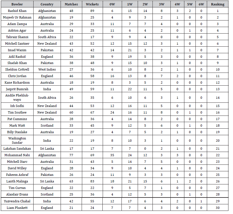
Table 3:Overall proportion (op) for the 7 wicket categories.

The James-Stein estimate of the optimal shrinkage constant for each *λ_i player is given in Figure 1 when the shrinkage target is 0.143. Lungi Ngidi has the maximum optimal shrinkage constant of 0.729 and has the highest shrinking towards the shrinkage target. Darren Sammy has the minimum optimal shrinkage constant of 0.033 and has the lowest shrinking toward the shrinkage target. The optimal shrinkage constant represents the confidence in our shrinkage target; a low shrinkage constant indicates more confidence in the baseline estimate given by the MLE. The empirical Bayes estimator pij is

Table 4 provides the parameter estimates of the concentration parametersα . Whileα <1 , provides sparse multinomial distribution, whileα >1 , provides smooth multinomial distribution. The values of the concentration parameters for the first five-wicket categories are higher than one, but for the last two wicket categories, the values are less than 1.

Table 4:Estimates of the concentration parameters and the shrinkage targets (j t ).

The estimates of the optimal shrinkage constants for the empirical Bayes method, where the shrinkage target is,

are given in Figure 2. Ashok Dinda has the maximum optimal shrinkage constant of 0.950 and has the highest shrinking towards the shrinkage target. Mohammad Nabi has the minimum optimal shrinkage constant of 0.663 and has the lowest shrinking toward the shrinkage target.

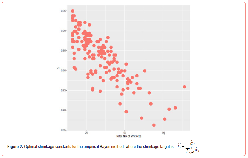
In the semi-parametric Bayesian approach, 100,000 draws were taken from a DP using Gibbs sampling with a burn-in of 50,000 under the following parameters:

Teh [8] proposed a formula to find the expected number of atoms in DP realizations based on α₀ and the number of observations. Based on that formula, we picked α₀ = 150, which provides reasonable no of clustering throughout the posterior simulations. For implementing the Bayesian regression model, we considered the following covariates: the number of overs the bowler bowled; the number of runs the bowler conceded in T20 matches from 1st of January 2010 to 11th of March 2020; type of bowler (0=‘Seam’, 1=‘Spin’); the age of the bowler and the economy rate of the bowler. For the age, we calculate the median age of the bowler for his playing period.

Figure 3 and Figure 4 provide the comparison of James-Stein (JS) shrinkage estimates with shrinkage target t_j=1/7 James-Stein (JS) shrinkage estimates with overall proportion (OP) as the shrinkage target, empirical Bayes (EB) estimates, maximum likelihood (ML) estimates, Dirichlet process (DP) estimates, Bayesian multinomial regression (BMR) estimates and overall proportions of wicket categories for different bowlers. The grey shaded area is the 95% credible interval of Dirichlet Process estimates. Here JS estimates are close to BMR estimates, whereas EB estimates are close to DP estimates, JS (OP) estimates, and ML estimates. The plots in the first row of Figure 3 are for the bowlers who got 6 wickets. We can see clearly, EB estimates and DP estimates are very close to the overall proportion. Rashid Khan and Ashok Dinda have wider 95% credible intervals of DP estimates since these two players don’t cluster with other players a lot, meaning those players have unique cell probabilities that differ from others.

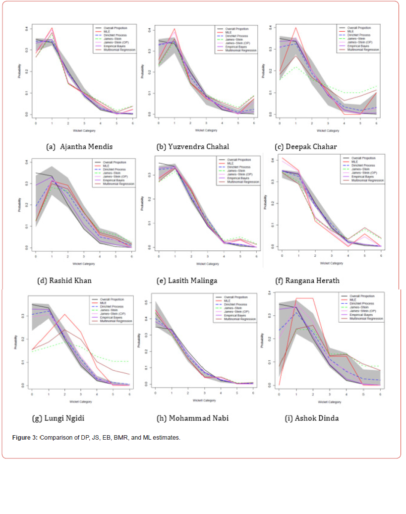
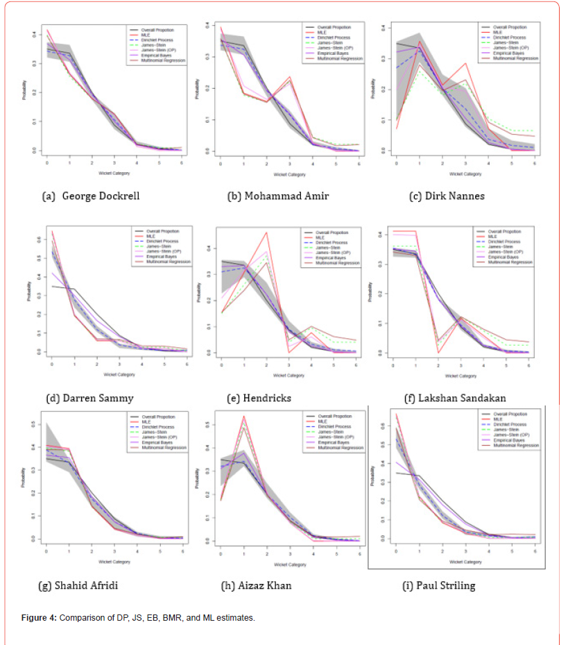
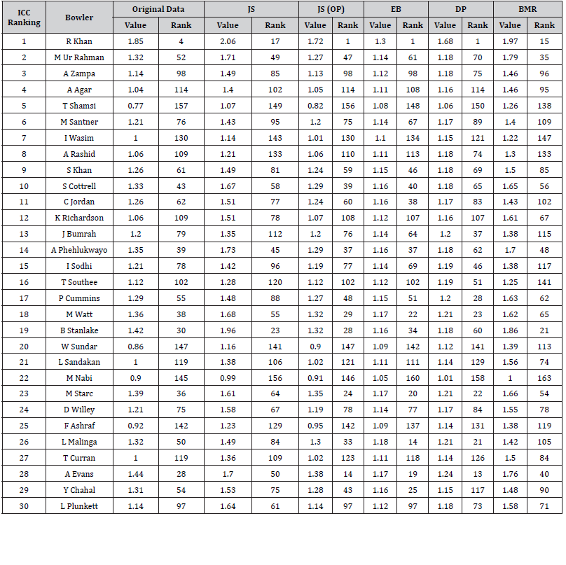
Table 5 provides the expected number of wickets per match based on estimates to assess the bowling performances of topranked bowlers. The ranks are given from the highest to the lowest value (the highest is rank 1), and the ties are given the highest rank using all the bowlers. Rashid Khan is the ICC top-ranked player and also the top wicket-taker who has the highest expected number of wickets per match (rank 1) based on estimates of James-Stein (JS) shrinkage estimates with overall proportion (OP) as the shrinkage target, empirical Bayes (EB) estimates and Dirichlet process (DP) estimates. However, Rashid Khan is given rank 4 based on the maximum likelihood (ML) estimates.

Table 5:Expected number of wickets per match for top-ranked bowlers.

Simulation Study

Although an in-depth simulation study is beyond what we originally set out to accomplish, it would be helpful to demonstrate and compare how the proposed and existing estimators perform over simulated datasets considering different scenarios. Nevertheless, we report here on a brief simulation study conducted using 10000 Monte Carlo simulations in two scenarios where the true cell probabilities are known. We report the Mean Squared Error (MSE) and compare the estimators below. Also, we varied the number of populations (m - 100, 200, and 500) and the number of categories (K5, 10, and 15) to explore the performance of the estimators. We generated data from multinomial distributions with sample sizes (ni) ranging from 15 to 75.

Scenario 1

In this first scenario, the true cell probabilities are strictly decreasing, but the differences between successive p’s are the same. For example, when K = 5, the true cell probabilities are

p =(5/15,4/15,3/15,2/15,1/15)   and that is used to generate the counts for all the populations. Table 6 provides the mean squared error values for each estimator based on Scenario 1. When m is fixed and K increases, the MSE decreases. The MSE also decreases when K is fixed and m increases. The proposed semi-parametric Bayesian estimator performs better than the existing estimators and MLE. This scenario is very similar to the cricket application, where the true cell probabilities of the wicket categories for each player generally have a decreasing pattern.

Table 6:MSE values for scenario 1.

Scenario 2

In the third scenario, the true cell probabilities increase and decrease (zig-zag pattern).

For example, when K = 5, the true cell probabilities are p =(1/23,10/23,1/23,10/23,1/23)

Table 7 provides the mean squared error values for each estimator based on Scenario 2. As in previous scenarios, when m is fixed and K increases, the MSE decreases. The MSE also decreases when K is fixed and m increases. Once again, the proposed semi-parametric Bayesian estimator performs better than the existing estimators and MLE.

Table 7:MSE values for scenario 2.

Discussion

In this paper, we considered four approaches for modeling bowling performance in T20I cricket. The advantage of the semi-parametric Bayesian approach is that it can accommodate complex and heterogeneous patterns in bowler performance. In particular, the Dirichlet process naturally borrows information across similar players and clusters them together. The cluster assignments of players are obtained as a by-product of the posterior simulation of the Dirichlet process. They are done in such a way that players have identical characteristics within clusters. The DP also seems to help in handling sparsity in the data as estimates for categories with zero counts for most players seem to behave appropriately.

We remark that choosing a suitable shrinkage target (tj) for James-Stein estimation is challenging. Two shrinkage targets we considered here were the discrete uniform distribution 1/K for all categories and the overall proportions. Data analysis suggests that shrinking towards 1/K is often less efficient than shrinking towards the overall mean proportion. Note that high shrinkage should generally be interpreted as a greater need to improve the MLE or as a greater lack of confidence in raw estimates based on past data, for instance, when based on small sample size. This being said, confidence in the shrinking target also plays a role here: raw estimates that align with a target tend to be shrunken more than others.

Table 8 provides the ranking based on the bowling statistics and estimates for the top 5 expected wicket takers per match. The total no of wickets and no of matches played are given after the bowler’s name in brackets, separated by a comma. The rank based on the expected wickets per match is given. Here we considered three bowling statistics; economy rate, bowling average, and strike rate, which are the popular statistics used to rank bowlers by ICC. The wicket-taking ability is high if the bowler has a lower economy rate, bowling average, and strike rate. The ranks for the bowling statistics are given from lowest to highest value considering all the bowlers. For example, Rashid Khan has the 2nd best bowling average out of all bowlers. Ashok Dinda has the highest wicket per match, but he played very few matches. Since he played a few games, it is clear that the ranking penalizes for the uncertainty, especially EB, through his performance being shrunk more towards the global shrinkage target. Rashid Khan has the highest rank for economy rate and bowling average compared to the other four bowlers. It seems that the Dirichlet process and empirical Bayes approaches rank these five bowlers in a more sensible way than the other approaches.

Table 8:Ranking based on bowling statistics and estimates for the top 5 expected wicket takers per match.

Availability of Data and Materials

All data generated or analyzed during this study are included in this published article.

Conflict of Interest

The authors declare that they have no competing interests.

References

1. Stein C (1956) Inadmissibility of the Usual Estimator for the Mean of a Multivariate Normal Distribution, University of California Press, Berkeley and Los Angeles (1956), Proceedings of the Third Berkeley Symposium on Mathematical Statistics and Probability 1: 197-206.
2. Ledoit O, Wolf M (2003) Improved estimation of the covariance matrix of stock return with an application to portfolio selection. Journal of Empirical Finance 10(5): 603-621.
3. James W, Stein C (1961) Estimation with Quadratic Loss, Proceedings of the Fourth Berkeley Symposium on Mathematical Statistics and Probability, pp. 361-379.
4. Hausser J, Strimmer K (2009) Entropy inference and the James-Stein estimator, with application to nonlinear gene association networks. Journal of Machine Learning Research 10: 1469-1484.
5. Efron B, Morris C (1973) Stein’s estimation rule and its competitors-an empirical Bayes approach. Journal of the American Statistical Association 68(341): 117-130.
6. Tvedebrink T (2010) Overdispersion in allelic counts and l-correction in forensic genetics. Theoretical Population Biology 200-210.s
7. Wadsworth WD, Argiento R, Guindani M, Galloway-PenaJ, Shelburne SA, et al. (2017) An integrative Bayesian Dirichlet-multinomial regression model for the analysis of taxonomic abundances in microbiome data. BMC Bioinformatics 18: 1-12.
8. Teh YW (2010) Dirichlet processes. Encyclopedia of Machine Learning.
9. Ferguson TS (1973) A Bayesian analysis of some nonparametric problem. The Annals of Statistics, pp. 209-230.
10. Blackwell D, Mac Queen JB (1973) Ferguson distributions via Polya urn schemes. The Annals of Statistics 1(2): 353-355.
11. Teh YW, Jordan MI, Beal M, Blei DM (2006) Hierarchical Dirichlet process. Journal of the American Statistical Association 101: 1566-1581.
12. Sethuraman J (1994) A constructive definition of Dirichlet priors. Statistica Sinica 4: 639-650.
13. Neal RM (2000) Markov chain sampling methods for Dirichlet process mixture models. Journal of Computational and Graphical Statistics 9(2): 249-265.
14. Swartz TB, Gill PS, Muthukumarana S (2009) Modelling and simulation for one-day cricket. The Canadian Journal of Statistics 37(2): 143-160.
15. Swartz TB, Albert J, Glickman ME, Koning RH (2017) Research directions in cricket. Handbook of statistical methods and analyses in sports.
16. Van Staden PJ, Cochran JJ, Bennett J, Albert J (2017) Cricket. The oxford anthology of statistics in sports 1: 2000-2004.
17. Silva R, Perera H, Davis J, Swartz TB (2016) Tactics for Twenty20 cricket. South African Statistical Journal 20(2): 261-271.
18. Davis J, Perera H, Swartz TB (2015) A simulator for Twenty20 cricket. The Australian and New Zealand Journal of Statistics 57(1): 55-71.
19. Koulis T, Muthukumarana S, Briercliffe CD (2014) A Bayesian stochastic model for batting performance evaluation in one-day cricket. Journal of Quantitative Analysis in Sports 10: 1-13.
20. Manage ABW, Scariano SM, Hallum CR (2013) Performance analysis of T20-world cup cricket 2012. Sri Lankan Journal of Applied Statistics 14: 1-12.
21. Van Staden PJ (2009) Comparison of cricketers’ bowling and batting performances using graphical displays. Current Science 96: 764-766.
22. Lemmer HH (2004) A measure for the batting performance of cricket players. South African Journal for Research in Sport, Physical Education and Recreation 26: 55-64.
23. Perera H, Davis J, Swartz TB (2015) Assessing the impact of fielding in Twenty20 cricket. Journal of the Operational Research Society 69(8): 1335-1343.