Factor and Cluster Analysis on the Evaluation of the Knowledge of use of Contraceptive Methods by Women in Nigeria.

Generally, the trend in this research is to use the quantitative measurement method and statistical curriculum and as well classify the scientific phenomena and analyse the reciprocal relation between phenomena by the basics objective, and the complications in most phenomena require the researcher to collect data for many variables, hence the collection of data is important in multivariate analysis methods, and in this method you need to understand and explain the interrelationships between the variables affecting the phenomenon.

Comparing the factor analysis with cluster analysis entails approaching a data collection from two opposing viewpoints. The basic rationale of both approaches is categorization. Classification in either approach is based on homogeneity. Classification in either technique is based on uniformity. Homogeneity in cluster analysis indicates that research units, which are positioned in the rows of the data matrix and might be individuals or groups of individuals, are categorised into clusters based on their similarity on variables. Clusters are best defined by object homogeneity within the cluster and object heterogeneity between clusters. Factor analysis, on the other hand, focuses on the homogeneity of variables that results from the similarity of values supplied to variables by respondents. Variables are located in the matrix’s columns and classified as factors or dimensions from the perspective of the data matrix [10].

Factor analysis (FA)

Factor analysis (FA) is a type of multivariate statistical method that focuses on data reduction and summarization. It deals with the problem of analysing the interdependence of a large number of variables and then explaining these variables in terms of their common, underlying factors.

The results and interpretations of methods are similar, but the mathematical models are different, so this method is a summary of the principal component (PCA) method [13]. The FA method is concerned with the correlations between a large number of quantitative variables. It reduces the number of primary variables by calculating a smaller number of new variables known as factors. This reduction is achieved by grouping variables into factors, which means that each variable within each factor is closely correlated, whereas variables belonging to different factors are less correlated [2, 13, 10, Sharma, 1996].

Factor model

Explains the factor model of observed variables (k) in sample size (n) by a linear function (m) of the common factors, where (m < k) and k is a unique factor for each variable namely that:

Where:
X: random vector of variables.
A: factor loadings matrix of any constant matrix.
F: random vector of common factors.
U: random vector of a unique factor.
μ: average vector

Basic assumption of factor analysis is the correlation between a variety of variables known as intra-correlation that affect by the existence of common factors and return to the reality of these factors, i.e., Cov(X_i,X_j)≠0,where the factor analysis explains these correlations that have minimum number of independent factors among them. These assumptions take the standard value of the variables, which are distributed normal distribution with mean (0) and variance (1), as well as to get rid of different variables and measurement units. Since the averages vector of both the common factor and unique factor are zero vectors depending on the assumption that the zero vector average variables:

The covariance matrix for each vector of the common factors (F) and the unique factors (U) (the assumption being independent) are as follows:

Under this assumption, we have three types of variation namely:
1. Common Variance is a part of the total variation and is correlated the rest of variables.
2. Specific Variance is a part of the total variation which in not correlated with the rest of variables but correlated with the same variable.
3. Error Variance is a part of exist variation during errors in the drawing of the sample or measured, or any other changes lead to volatility in the data.

Share all of the common’s variation, specific variance, and error variance to create in the total variation which represents the equation.

The square roots of common ratios of a_j1 to a_jm to return loading factors and represents the amount of the correlate of variable j for each factor [2, 14].

The communalities of the variable j (standard value) are the sum square of factors loading analysis of variable and represents the variation ratio which interprets summary factors from the correlation matrix analyzed for these variables, and symbolized by the symbol and the following formula: h_j²

Where:
a_jp represents a weight of factor p for variable j which a matrix of factors known in factors loading. Therefore, the total variation of the variable j represents by equation.

Where: s_j represents the total variation that is associated to each variable. One characteristic of h_j²

The extent h_j² of overlap between the variables and summary factors: if h_j² is large and close to one, this means that the variable interferes with summary factor. If h_j² is equal to zero, it means that the summary factor is not able to explain any part of the variation. If h_j² is between zero and one that indicate the partial overlap between the variables and factors. [13, Sharma, 1996].

Principal components analysis is a technique for transforming variables in a multivariate data set into new variables that are uncorrelated with each other and account for reducing proportions of the original variables’ total variance (Sharma, 1996). Each new variable is defined as a linear combination of the old ones. The method is described in detail in [5] but in summary. The first principal component, 1 PC , is defined as the linear combination of the original variables, x₁,x₂, ,− − − x_k, that accounts for the maximal amount of the variance of the x variables amongst all such linear combinations [2, 1].

The second principal component, 2 PC , is defined as the linear combination of the original variables, x₁,x₂, ,− − − x_k that accounts for a maximal amount of the remaining variance subject to being uncorrelated with 2 PC . Subsequent components are defined similarly.

The matrix of data x_n×m contains (m) columns of variables and (n) rows of observations. Matrix of data calculated by correlation matrix and the application of PCA by the correlations matrix to get m of characteristic roots that symbolizes by λ_i in decreasing order λ₁>λ₂ > − − −λ_m which represent variations of summary factors. [2, 1].

Explain of characteristic vector placed as factors in the linear combination of the original variables to give ( ij PC ) of the value i of the principal component j: -

Where: PC_ij represents the principal component j, a_ij represents the coefficient of variable (i) of the component (j) which are values of Eigen Vectors accompanying of Eigen roots.

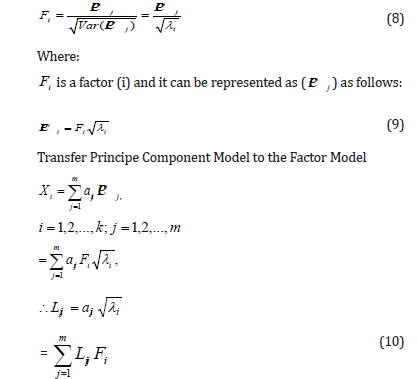
In the correlation matrix user, the variation j equal to Var ( PC_ij )=λ_i and λ_i represents a characteristic root of the principal component j. It can be obtained by summary factors to get factors F₁,F₂,...,F_m by dividing each principal component of the standard deviation as follows:

After obtaining the initial factor solutions, one is interested to rotate the loadings. The goal of factor rotation is to find simpler factor structure that can use to make interpretation of the resulting factors easily and meaningfully and to determine the appropriate number of factors. It is a way of maximizing high loadings and minimizing low loadings so that the simplest possible structure is achieved. To accomplish this and for the simplicity of this study, orthogonal rotations are done using the varimax procedure. Here we only focus on the orthogonally rotated solutions as they can produce more simplified factor structures from a large amount of data [13, 5; Sharma, 1996; 3].

In this research we used loading method by orthogonal method (Kaiser - Varimax) that applies the definition of the variation by factor loading (i).

Where:
Var (F_k) represents a variation factor (k), a_jk represents the value of the saturation variable (j) factor (k). p represents the number of variables.

Choosing the number of factors

It is crucial to pick the right number of common factors. We make a graph pair ( j j,λ ), (the “scree plot”) and watch for when it starts to become “flat” (Cattell, 1966). The Kaiser criterion is another criterion for dealing with the number of factors issue (Kaiser 1960). When the eigenvalues are greater than one (λ>1), a factor j is important. If the number of factors discovered by the Kaiser Test is equal to the number of factors discovered by the “scree plot,” we can proceed with the other procedures; otherwise, we must choose one of the previously obtained results. If one of the produced results from the “scree plot” graphic is chosen, the preceding methods must be performed in order to arrange the best number of elements. As the number of factors increases, so do the results. Optional methods include Kaiser’s (Kaiser 1956) “eigenvalues greater than one” rule, the scree plot, a priory theory, and preserving the number of components that accounts for the greatest proportion of variance or provides the best interpretable solution [13, 12].

Variance extracted

Another strategy based on a similar conceptual structure is to keep the number of components that account for a particular percentage of the retrieved variance. The research differs on how much variance must be explained before the number of components is considered sufficient. The majority believes that 75-90% of the variance should be accounted for; however, some believe that as little as 50% of the variance explained is acceptable. This seemingly broad norm must be examined in connection to the fundamental distinctions across extraction methods, as with any criterion method that is primarily based on variance. When evaluating the value of percent of variance extracted, the amount of variation that was included for extraction must be considered [3]. Component analysis contains more variance to be described, implying that higher percentages of explained variance are expected than would be required if only common variance is included [3].

Cluster analysis is a class of multivariate techniques that aims at grouping objects or respondents based on the characteristics they have (Malhotra & Birks, 2007; Hair et al. 2009). The clusters formed based on the analysis should demonstrate high homogeneity within clusters and high heterogeneity between clusters. Cluster analysis differs from factor analysis in the sense that the former is concerned with reducing the number of objects by grouping them into clusters whereas the latter aims at reducing the number of variables by grouping them to form new constructs or factors [5, Sharma, 1996].

The first task in cluster analysis is to select the variables that are used for forming clusters. The selected variables should be meaningful in describing the similarities between objects in consideration of the research questions.

There are two key assumptions with regard to cluster analysis. The most important one states that the basic measure of similarity, which is the basis of clustering, must be a valid measure of the similarity between objects. A second major assumption is that there is theoretical justification for structuring the objects into clusters. These two assumptions are both valid for my data set and will be used in the following analysis [5, Sharma, 1996].

Element

Element (X_i) is a vector distance for measurement for the n-dimensional Xi=(X_i1,X_i2,...,X_in) and elements are numerical amounts of possible measurement (Yan,2005).

A. Element selection

The goal of cluster analysis is to investigate the cluster structure in data without knowing the true categorization. The elements chosen for research will, in particular, define the data structure. The underlying clusters or populations should be represented by an ideal sample. Outliers (datapoints that fall outside the general region of any cluster) should be avoided as much as possible in order to ease the recovery of distinct and trustworthy cluster structures, even if they do occasionally form a single cluster (Yan, 2005).

B. Variable selection

Data investigated in cluster analysis are often recorded on multiple variables. The importance of choosing an appropriate set of variables for clustering is obvious (Yan, 2005).

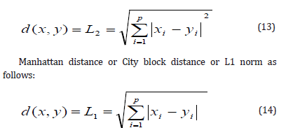
An essential step in the cluster analysis procedure is to obtain a measure of the similarity or “proximity” between each pair of objects under study. The Minkowski metric or Lq norm calculates the distance d between the two objects x and y by comparing the values of their n features. The Minkowski metric can be applied to frequency, probability and binary values [13, 9].

Where:
d(x,y) is the distance between x and y and
p is the number of variable
s Two important special cases of the Minkowski metric are q=1and q=2. The most commonly used measure of similarity is Euclidean distance or L2 norm, which can be expressed as follows:

Cluster

Is a collection of adjacent elements in the statistical community and homogenous to some extent, also known as a group of similar things, that are different from the other clusters [9].

To visualize the clustering results various versions of the dendrogram have been proposed and widely used. The main objective of this visualization is a tree-based structure yielded by a hierarchical algorithm which is easy to understand the similarities/ dissimilarities between elements. It demonstrates both the cluster and the sub-cluster relationships and also the order in which the clusters are merged for agglomerative algorithm or split for divisive case. Usually, a dendrogram is read from left to right. In a dendrogram, the data points are represented along the bottom and referred to as external/terminal nodes, and clusters to which the data belong are formed by joining with the internal nodes. The name of objects added to the terminal nodes are known as labels. The height of the dendrogram shows the distance between objects or clusters. Therefore, the small values of the height indicate a high similarity between the objects and the large value of the height indicates more distance. This can be shown in the figure below. The coalition between each internal node and the height can be explained mathematically by the following condition: [13, 9].

For every subset of objects Q and R and Q ∩ R ≠ Φ Here, h (Q) and h(R) represent the highest of Q and R respectively.

The focus was on hierarchical cluster which was summarized by [8] and are employed in this study:

Cluster analysis is a technique for identifying trends in a data collection by grouping (multivariate) observations into clusters. Hierarchical clustering is one of the cluster analyses approaches because it involves grouping and categorizing data into clusters, and these clusters are very similar to each other in terms of similarity within clusters, but they differ or are dissimilar between clusters. Hierarchical cluster analysis is regarded as a good, active method and tool for analysing data in various ways. This method (Hierarchical cluster) is used to analyse a data matrix that consists of (n) elements, each of which has a number of variables (p). Hierarchical approaches are classified into two types: agglomerative and divisive [13, Shen, 2007].

Agglomerative hierarchical clustering begins with n clusters, each containing a single object in the data. The two clusters with the shortest between-cluster distances are fused in the second phase, and they will be considered as a single cluster in the following step. As the operation progresses, a single cluster holding all n objects is formed.

The divisive approach goes in the opposite direction. That is, it starts with a single cluster with all the data points in it, and iteratively divides it into two clusters that are furthest apart from one another.

The structure in (Figure B) resembles an evolutionary tree, and it is in biological applications that hierarchical classifications are perhaps most relevant. According to Rohlf (1970), a biologist, „all other things being equal‟, aims for a system of nested clusters.

Agglomerative hierarchical clustering algorithm steps in below
 compute the distance matrix.
 Repeat
 Merge the closest two clusters.
 Update the distance matrix to reflect the proximity between the new cluster and the original clusters.
 Until only one cluster remains.

There are two types of clustering methods such as Nearest Neighbor (Single Linkage) and Furthest Neighbor (Complete Linkage):

The distance d between two clusters C_i and C_j is defined as the minimum distance between the cluster objects. The cluster distance measure is also referred to as single linkage. Typically, it causes a chaining effect concerning the shape of the clusters, i.e., whenever two clusters come close to each other they stick together even though some members might be far from each other [13].

The maximum distance between cluster objects is defined as the distance d between two clusters Ci and Cj. Complete-linkage distance is another name for cluster distance. Because every object within a cluster is expected to be adjacent to every other object within the cluster, and outlying objects are not incorporated, it typically creates compact clusters with tiny widths (Yim & Ramdeen, 2015).

The loss of information (or increase in inaccuracy) while merging two clusters is defined as the distance d between them (Ward, 1963). The sum of distances between the cluster’s objects and the cluster centroid cenC is used to calculate the error of a cluster C. When two clusters are combined, the combined cluster’s error is greater than the sum of the errors of the two individual clusters, resulting in information loss. However, the merging is done on the most homogenous clusters in order to unite them and reduce the amount of variation within the merged clusters. Ward’s approach is prone to producing small, compact clusters. It is a least squares method, so implicitly assumes a Gaussian model (Sharma, 1996).

This part includes the application of two types of multivariate analysis (factor analysis and cluster analysis) to identify the most important method of modern contraceptives among married women and the comparison between the results of the analyzes in order to know the extent of conforming between them. Results were extracted using the statistical program (SPSS V.22).

The data used for this research was a secondary data extracted from the National Population Commission (NPC 2020). The information on the knowledge and use of family planning methods was obtained from female respondents by asking them to mention any ways or methods by which couple delay or avoid pregnancy. However, the actual sample size used in analysis is 7,621.

Results of factor analysis

The contraceptives indices used in this study were numbered as follows:
1. No method,
2. Female sterilization,
3. Male sterilization,
4. Any method,
5. Any traditional methods,
6. IUD,
7. No of women age 15-49 years currently married or in union,
8. Any modern method,
9. LAM,
10. Others,
11. Withdrawals,
12. Periodic abstinence,
13. Injectables,
14. Diaphragm,
15. Implant,
16. Female condom,
17. Male condom,
18. Pills.

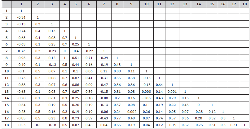
(Table 1) shows the correlation matrix which is typically used as an eyeball test and gets a feeling for which variable is strongly associated with which variable.

Table 1: The correlation matrix.

(Table 2) provides the Kaiser-Meyer- Olkin (KMO) and Bartlett’s test of sphericity. The KMO criterion can have values between (0,1) where the usual interpretation is that 0.8 indicates a good adequacy to use the data in a factor analysis. If the KMO criterion is less than 0.5 we cannot extract in some meaningful way. However, the overall Measure of Sampling Adequacy (MSA) for the set of variables included in the analysis was 0.565, which exceeds the minimum requirement of 0.50 for overall MSA and also means this test does not find the level of correlation to be too low for factor analysis. The variables remaining in the analysis satisfy the criteria for appropriateness of factor analysis.

Table 2:KMO and Bartlett’s Test.

(Table 3) which is the next table is the Anti-image Matrices. The image theory splits into image and anti-image. The rule of thumb is that in the anti-image covariance matrix only a maximum of 25% of all non-diagonal cells should be greater than (0.09).

Table 3:Anti-image Matrices..

Anti-image Covarian

The second part of the table is the anti-image correlations where the diagonal elements of that matrix are the MSA values. A figure of 0.8 indicates good accuracy; if MSA is less than 0.5, we exclude the variable from the analysis. We find that those who took pills has a MSA value of 0.370 and might be a candidate for exclusion, we can proceed with our factor analysis.

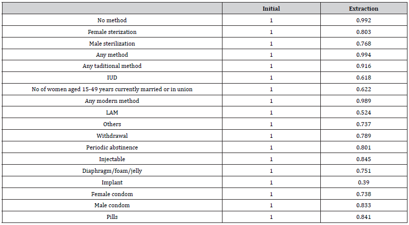
The next which is Table 4 shows the communality. The communality of a variable is the variance of the variable that is explained by all factors together. Mathematically it is sum of the squared factor loadings for each variable. A rule of thumb is for all communalities to be greater than 0.5. This holds true in this example, for all the communalities are greater than 0.5 as can be seen in the above table.

Table 4:The communalities.

(Table 5) shows the proportion of variability which is firstly explained with all factors together and then only with the factors before rotation. The table also includes the eigenvalues of each factor. The eigenvalue is the sum of squared factor loadings for each factor. SPSS extracts all factors that have an eigenvalue greater than 0.1. The result shows five factors. The table also shows us the total explained variance before and after rotation. The rule of thumb is that the model should explain more than 70% of the variance. In this study, the model explains 77% (Figure 1).

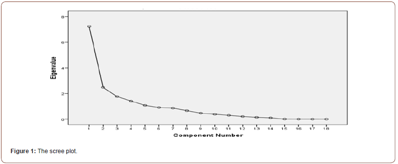
Table 5:Total Variance Explained.

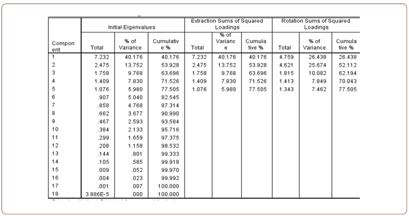
Extraction method: Principal Component Analysis

The scree plot graphs the eigenvalue against the factor number. We can see the value of the first and second column of the table immediately above. From the second factor on, we can see that the line is almost flat, meaning that each successive factor is accounting for smaller and smaller amounts of the total variance.

(Table 6, 7) which displays the factor matrix, and the rotated factor matrix are the keys in interpreting our factor. The factor loadings that are shown in the tables are the correlation coefficient between the variable and the factor. The factor loadings should be greater than 0.4 and the structure should be easy to interpret.

Table 6:The Factor Matrix.

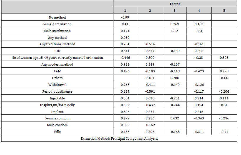
Table 7:Rotated Factor Matrix.

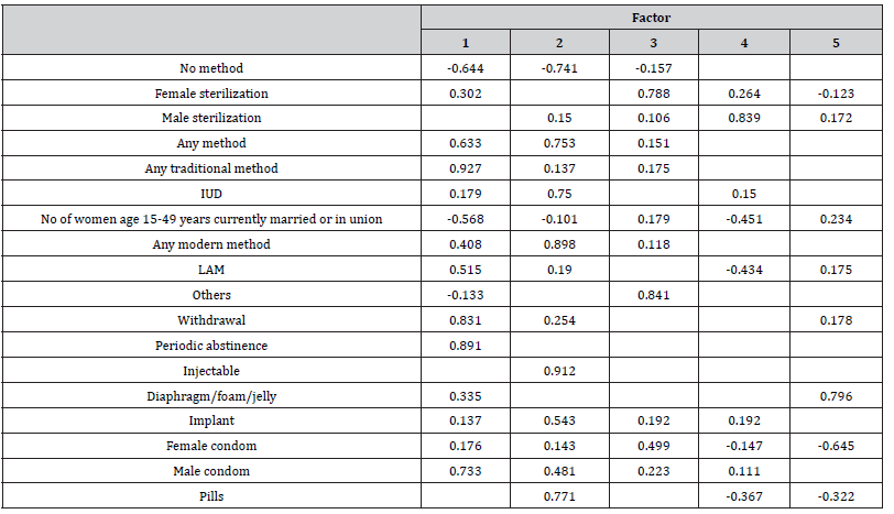
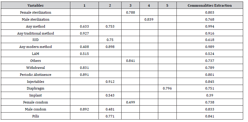
For analysis and interpretation factor analysis result in (Table 6, 7) we are only concerned with rotation sums of squared loadings. Here note that the first factors explain relatively large amounts of variance for 36.7% of the total variance and included seven variables (Any method, Any traditional method, Any modern method, LAM, Withdrawal, Periodic abstinence, male condom), the second factor explained 36.7% of the total variance and contain seven variables (Any method, IUD, Any modern method, Injectables, Implant, Male condom and Pills), the third factor has been interpreted 16.0% of the total variance with variables (Female sterilization, others and Female condom), the fourth factor explains 5.3% of the variance and included one variable (Male sterilization) and factor five explains 5.3% of the total variance and contain variable (Diaphragm). All the remaining factors are not significant.

The Results of cluster analysis

Cluster analysis was used to determine the relationship between the variables studied in terms of the degree of similarity or difference and classify of the variables into homogeneous groups among them. Cluster analysis has been used to classify variables that evaluates the use of contraceptives by women into five clusters separately which is the strong degree of homogeneity among the members of one cluster and weak between members of different clusters. We have used Ward’s Method among the methods of cluster analysis and have used Euclidean Distance measure to create the matrix distance. The results were as shown in the (Figures 2, Table 9).

Table 8:Rotated factor matrix and communalities.

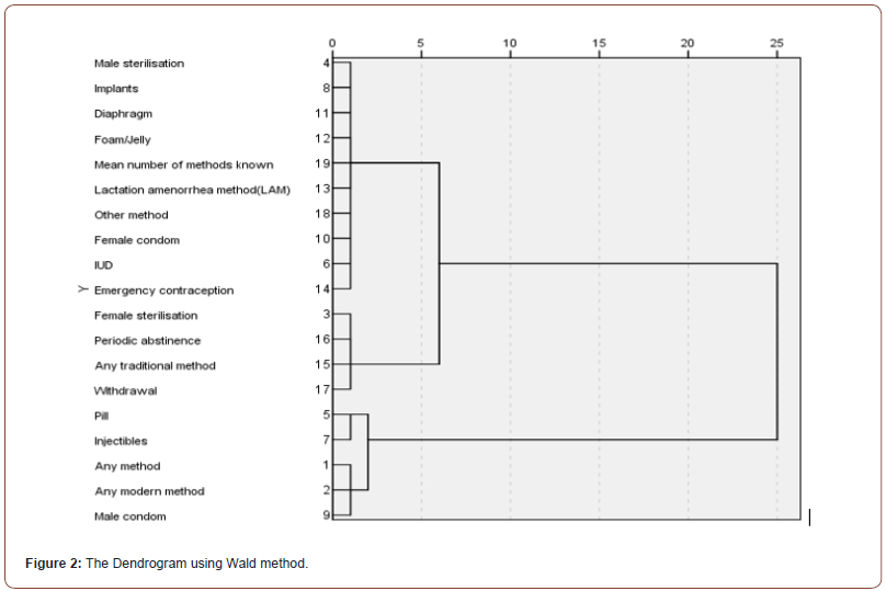
(Figure 5) shows five number of clusters that used in this analysis as well as variables belong to each cluster. Vertical axis (Y) in the structure represents the distance between merge variables and the horizontal axis (X) represents the merge variables. (Table 9) indicates the number of clusters and the proportion of variables within each cluster as well as variables within each cluster.

Table 9:Cluster analysis of data.

A comparison of the results of factor analysis and cluster analysis

Table 10:Comparison between the results of factor analysis and cluster analysis.

(Table 10) contains a comparison between factor and cluster analysis of the data in order to determine the compatibility of the results of analyses, which illustrate the number of variables in each factor as same as number of variables in each cluster and both analyses gave the closest results.

Cluster analysis showed the lowest distance between Any method and any modern method is 4.825 while the highest distance between Withdrawal method and Periodic Abstinence is 9,568.173 as well as factor analysisin table 1 shown, the highest correlation between Any method and any modern methodis 0.957 while the lowest correlation between withdrawal method and Periodic Abstinence is 0.638.

Conclusion

The most important conclusions were summarized through practical part as follows:
1. The analysis shows that there are quite similarities between the results of factor analysis and cluster analysis which the number of factors equal to the number of clusters, as well as in terms of inclusion, the factor analysis and cluster analysis have the same variables in each cluster and factor with the same sequence except the factor and cluster 4, 5 with difference place of variables.
2. Both results show that there are five significant factors and five important clusters from which to determine the variables in evaluating the use of contraceptives the ratio explain is 77.5% of the total variance.
3. The lowest distance is between Any method and any modern method while the highest distance is between Withdrawal method and Periodic Abstinence as well as the lowest correlation is between Any method and any modern method while the highest correlation is between Withdrawal method and periodic abstinence.
4. In this research reveals that
1. The contraceptives prevalence rate is 15% among currently married women using Any method of contraception.
2. Any method, any modern method, Withdrawal, Periodic Abstinence were mostly used in Nigeria.
3. Family planning with the use of traditional method of contraceptive in Nigeria is very low.

Recommendations

1. We recommend the possibility of using factor analysis in the classification gives the same results as cluster analysis, especially when the application analyzes.
2. Taking into account the findings of a study of use of contraceptives in family planning and try to be educated, campaigned and encourage couples to limit or space the number of children they want to have through the help of government via Health sectors.
3. Comparisons to be made between other methods of cluster analysis and the other ways the factor analysis.

None.

No conflict of interest.

1. Johnson R A, Wichern D W (2013) Applied Multivariate Statistical Analysis, (6^th), Pearson Prentice Hall.
2. Rencher A C (2002) Methods of Multivariate Analysis, Second edition, Brigham Young University, John Wiley & Sons, Inc, USA.
3. Anderson T W (1984) An Introduction to Multivariate Statistical Analysis, (2^nd ), John Wiley and Sons, New York-U.S.A.
4. Seber G A F (1984) Multivariate Observations. John Wiley and Sons, New York - USA.
5. Everitt B S (2005) An R and S-PLUS Companion to Multivariate Analysis, Springer-Verlag London.
6. Afifi A, Clark V (1984) Computer Aided Multivariate Analysis, Lifetime Learning Publications, USA.
7. Beavers A S (2013) Practical Considerations for Using Exploratory Factor Analysis in Educational Research 18: 6.
8. Muca M, Puka L, Bani K (2013) Principal Components and the maximum likelihood method as tools to analyze large data with a psychological testing example, European Scientific Journal 9(20): 176-184.
9. Hair JR (2010) Multivariate Data Analysis, Seventh Edition, Pearson Prentice Hall.
10. Han J, Kamber M, Pei J (2012) Data Mining “Concepts and Techniques”, (3^rd), Morgan Kaufmann, USA.
11. Clatworthy J, Deanna Buick, Matthew Hankins, John Weinman, Robert Horne, et al. (2005) The use and reporting of cluster analysis in health psychology: A review. British Journal of Health Psychology, 10(3): 329-358.
12. Everitt B S (2011) Cluster Analysis. Chichester, UK: John Wiley & Sons, Ltd.
13. Finch H (2005) Comparison of distance measures in cluster analysis with dichotomous data. Journal of Data Science 3(1): 85-100.
14. Kaufman L, Rousseeuw P J (1990) Finding Groups in Data “An Introduction to Cluster Analysis”, John Wiley and Sons.