


 Review Article
Deep Learning Signal Processing
Received Date:February 15, 2025; Published Date:February 25, 2025
Abstract
This article focuses on deep learning for random and normalian variables to which we associate toxic and non-toxic characteristics randomly as well. I will give the definition of forward propagation, the definition of back propagation, and also the definition of a two-layer neural network. The results obtained are an image containing toxic and non-toxic samples classified into two groups, I will also give as results the learning curve and the accuracy curve. At the end of this article, I will give the python script that made it possible to obtain these results.
Keywords:Deep learning; normalian variable; toxic; non-toxic; forward propagation; back propagation; neural network; learning curve; accuracy curve
Introduction
Deep learning is a critical subfield of AI (Artificial Intelligence). It is based on machine learning through complex neural networks. This advanced field of machine learning can lead to a deeper understanding of algorithms designed from the neural network of the human brain. Deep Learning makes it possible to achieve complex objectives, ranging from computer vision, object recognition within images, neuro-biological data processing… etc. Deep learning is a rapidly evolving technology as its algorithms interact with complex data by learning to make decisions autonomously and from unstructured data. This allows for no human intervention, unlike machine learning, which requires human intervention to learn the decision- making methodology from large amounts of data. Deep learning is a branch of machine learning that relies on the architecture of artificial neural networks without human intervention, unlike machine learning, which requires human intervention in order to learn the learning methodology.
Artificial Neuron
A neuron can be schematized as shown in the following Figure 1.
A neuron is the basic processing unit of a neural network. It is connected to input sources of information (e.g., other neurons) and returns information as output.
Forward Propagation
For a 2-layered neural network, [1,5] the forward propagation is summarized by the calculation of matrices Z[3] and A[3] as shown below Figure 2.

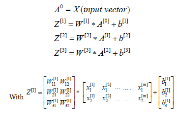
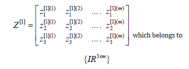
And therefore, Z can be written in matrix form as indicated by the following formula:
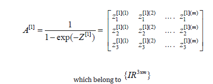
Similarly, we give the activation function in matrix form as follows:
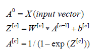
Generalizing, we have the following formulas:
Where:
c is the index of the neuron layer
A[c] , W[c] and b[c] are the matrix form of the activation, of
the weighting functions and the noise vector, all that respectively
correspond to the layer c.
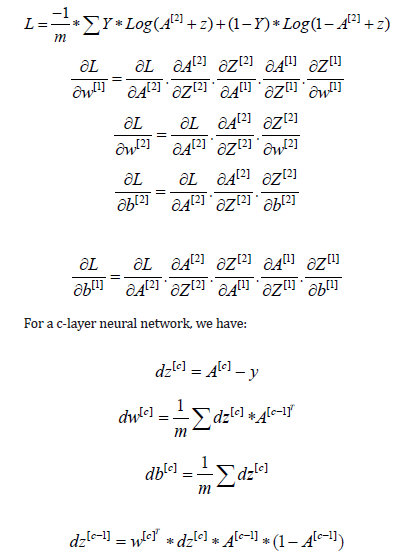
The Log Loss Function to Minimize and Back Propagation
The cost function [3,4] to be minimized is given by the following formula:
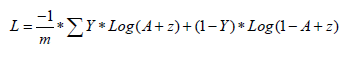
Where Y is the binary variable known as a vector of dimension m.
Then comes the optimization to minimize the cost function by going through the descent of the gradient. Gradient decent, and updated W and b (noise) parameters are the back propagation such as:
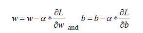
The optimization process is based on the Gradient decent and on the updated of W and b (noise). This optimization process is such:

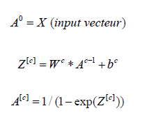
For a c-layered neural network, the forward propagation is summarized by the calculation of matrices Z[c] and A[c] as shown below:
Where:
c is the index of the neuron layer.
A[c] , Wc are respectively the matrices of activation and of
weighting functions at layer c
bc is the noise vector corresponding to layer c
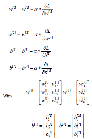
Next comes the partial derivatives of the Log Loss cost with respect to w and b for two layers:
For a c-layer neural network, we have:
Algorithm of Deep Learning
Learning Curve
The obtaining learning curve (Figure 3) is downward at the beginning and flat towards the end for these data, with the cost per unit represented on the Y axis and iterations index on the X axis. As learning increases, the cost per unit of output initially decreases before flattening as it becomes more difficult to increase the efficiency gained through learning process.


Validation Curve
Exactitude measured by the deviation of the results from the “true” value. Combination of fidelity and exactitude Y is the total error. It is not because we have a faithful and fair method that it is automatically exact [2,6]. It is therefore necessary to check the exactitude at the end Figure 4. Exactitude is a metric for evaluating the performance of classification models with 2 or more layers. Exactitude can be translated as “precision” in French. Like other metrics, exactitude is based on the confusion matrix. As a reminder, the confusion matrix is composed of 4 values (True Negative, False Negative, False Positive, True Positive).

Deep Learning Image Result
Accuracy makes it possible to describe the performance of the model on positive and negative individuals in a symmetrical way. It measures the rate of correct predictions on all individuals Figure 5.
Conclusion
Machine learning and deep learning are two types of artificial intelligence (AI). Machine learning is AI that can adapt automatically with minimal human interference, and deep learning is a subset of machine learning that uses neural networks to mimic the learning process of the human brain. Our algorithm uses Deep Learning to classify input data into two groups, toxic and non-toxic samples, as shown in Figure 5.
Deep Learning vs Machine Learning: What Are the Differences?
Machine learning and deep learning are two types of artificial intelligence. Machine learning is AI that can adapt automatically with minimal human interference, and deep learning is a subset of machine learning that uses neural networks to mimic the learning process of the human brain. There are several major differences between these two concepts. Deep learning requires larger volumes of training data, but learns from its own environment and mistakes. On the contrary, machine learning allows training on smaller datasets, but requires more human intervention to learn and correct mistakes. In the case of Machine Learning, a human must intervene to label the data and indicate its characteristics. A deep learning system, on the other hand, tries to learn these characteristics without involvement.

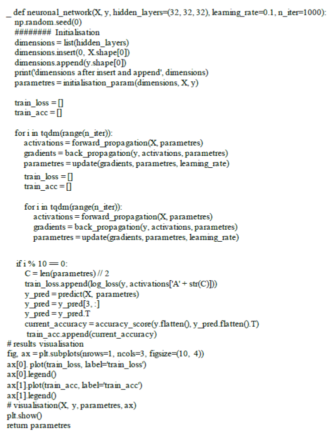
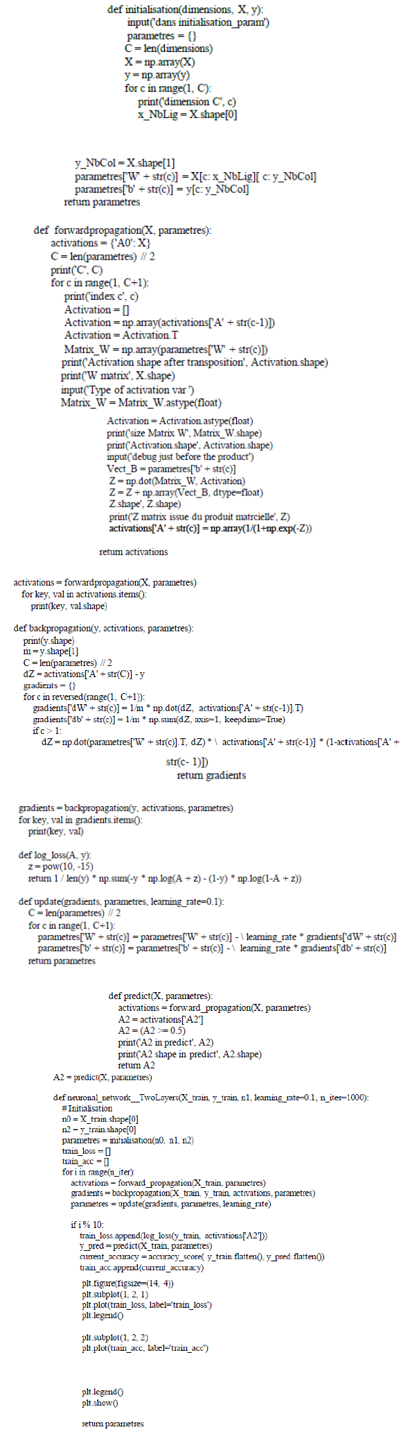
Script With Python Language
References
- Amita Kapoor, Antonio Gulli, Sjit Pal, François Colled (2022) Deep Learning with Tensor Flow and Keras. Third Edition: Build and deploy supervised, unsupervised deep, and reinforcement learning models.
- Catherine Y (2015) Exactitude et intervalles statistiques en validation de mé 17th International Congress of Metrology.
- Collobert R (2011) Deep learning for efficient discriminative parsing. Artificial Intelligence and Statistics 15: 224-232.
- Amitha M, Arul A, Sivakumari S (2021) Deep Learning Techniques: An Overview. Advanced Machine Learning Technologies and Applications PP. 599-608.
- Schmidhuber J (2015) Deep learning in neural networks: An overview. Neural Networks 61(3): 85-117.
- Gulshan V, Peng L, Coram M, Stumpe MC, Wu D, et al. (2016) Development and Validation of a Deep Learning Algorithm for Detection of Diabetic Retinopathy in Retinal Fundus Photographs. JAMA 316(22): 2402-2410.
-

This work is licensed under a Creative Commons Attribution-NonCommercial 4.0 International License.


